Statistics Final Exam Review: Chapters 6-9

Comprehensive vocabulary flashcards covering statistical inference, hypothesis testing, and linear regression principles based on the lecture notes.

Sampling Variability

The phenomenon where different random samples from the same population produce different statistics, reflecting uncertainty in statistical inference.

Sampling Distribution

A distribution showing how a statistic varies across repeated samples; it is a key tool used to construct confidence intervals and test hypotheses.

Sample distribution

the distribution of the values in one observed sample, described by x, s

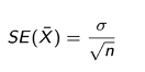
Standard Error (SE)

SE measures the spread of a sample statistic (e.g. ¯X) around the true parameter — i.e. the precision of the estimate.

Standard deviation

SD (σ or s) measures the spread of individual observations around their mean. It describes variability in the data.

Central Limit Theorem (CLT)

A theorem stating that for a large sample size ($n > 30$), the sampling distribution of the sample mean $\bar{X}$ is approximately normal.

Point Estimation

The use of a single value, such as a sample mean $\bar{X}$ or sample variance $S^2$, to approximate an unknown population parameter like $\beta$ or $\text{σ}^2$.

Interval estimation

giving a range of plausible values for the parameter, explicitly acknowledging sampling uncertainty

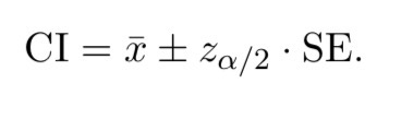
Confidence interval (CI)

a specific interval estimate with a stated confidence level. A 95% CI means: if we repeated the sampling many times and built an interval each time, about 95% of those intervals would contain the true parameter.

Unbiasedness

A property of a point estimator where the estimator is correct on average.

Consistency

A property of a point estimator where the estimator converges toward the true population parameter as the sample size increases.

Null Hypothesis ($H_0$)

The default assumption in hypothesis testing representing no effect, no difference, or no relationship; failing to reject it does not prove it is true.

Alternative Hypothesis ($H_1$)

The competing claim in hypothesis testing that represents what the researcher is looking for evidence of; it is the opposite of the null hypothesis.

Types of hypothesis tests (shaded tail regions represent the rejection regions)

o  Two-tailed test → looking for any difference (H₀: μ  = 50 ; H1: μ ≠ 50)

o  Right-tailed test → looking for an increase (H₀: μ < 50 ; H1: μ > 50)

o  Left-tailed → looking for a decrease (H0 μ > 50 ; H1: μ < 50)

p-value

A measure of how likely the observed sample result is if the null hypothesis is true; used to make decisions by comparing it to the significance level $\text{α}$.

Two equivalent approaches

critical value approach: compute the test statistic; reject H₀ if it falls in the rejection region (e.g. |z| > z_α/2 → Reject H₀ )

p-value approach: Compute the p-value (probability of data this extreme if H0 true); reject H0 if p<α.

Type I Error

A false positive error that occurs when the researcher rejects the null hypothesis $H_0$ when it is actually true.

Type II Error

A false negative error that occurs when the researcher fails to reject the null hypothesis $H_0$ when it is actually false.

Test Power

The probability of correctly detecting a true effect, calculated as $1 - \text{β}$, where $\text{β}$ is the probability of a Type II Error.

Power rises with larger n, larger effect size, and larger α

Purpose of preliminary inferential analysis

before estimating a full model, preliminary inference checks the basic statistical features of the data — whether variables differ across groups, whether relationships exist, and whether modelling assumptions are reasonable. It guides specification and prevents naive modelling

Examples: one sample t-test, two sample t-test, one way anova

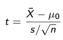
One-Sample t-test

A test used to compare the observed sample mean with a known benchmark value to assess if the difference is larger than sampling uncertainty.

Interpretation:

o   Small p-value: evidence against benchmark

o   Large p-value: difference reflects random variation 

o   Rule of thumb: Large absolute t-statistics (+/- 2) indicate strong evidence against benchmark

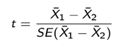
Two-Sample t-test

A test used to compare the average outcomes of two groups to evaluate if the observed gap is larger than sampling noise.

Interpretation:

o   Small p-value: groups differ significantly

o   Large p-value: gap may simply reflect noise

o   Rule of thumb: Large absolute t-statistics (+/- 2) indicate strong evidence

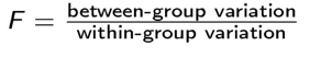
One-Way ANOVA

A statistical test that evaluates whether multiple groups have the same average outcome, though it does not identify which specific groups differ.

Interpretation:

o   Small p-value: at least one group differs

o   Compute F-statistic and p-value

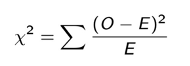
Chi-Squared Test

A test used to compare observed category frequencies with expected frequencies to determine if there is a statistical association between categorical variables.

Interpretation:

o   Small p-value: evidence of association between categories

o   Large p-value: observed differences in frequencies may reflect random variation

o   Large x²-statistics indicate strong evidence of association

General Equilibrium (GE)

An economic framework that looks at the whole economy where all markets affect each other and balance simultaneously.

Partial Equilibrium (PE)

Looks at just one market or a few variables, assuming everything else in the economy stays the same.

Ceteris Paribus

A Latin phrase meaning "all other things being equal," used to study the relationship between two variables while keeping other factors constant.

Purpose of a regression model

o   links an outcome variable Y to explanatory variables X

o   estimates the direction and magnitude of relationships

Correlation (r)

is a unit-free, symmetric measure of linear association between two variables, bounded in [−1,1].

regression slope (β) - regression coefficients

has units (change in Y per one-unit change in X), is not symmetric (X on Y differs from Y on X), and in multiple regression measures the effect of X holding other variables constant.

Adjusted R²

proportion of the variation in Y explained by the model (0 ≤R²≤1). If R² = 1 then it is perfect model fit.

Adjusted R² penalizes unnecessary variables and only increases when a new variable improves the model enough.

- Penalizes adding irrelevant variables

- prevents improvement from ad-hog regressors

- High R² does not guarantee reliable model, because some variables are unnecessary

Ordinary Least Squares (OLS)

An estimation approach that determines the "best" parameter values by minimizing the sum of the squared prediction errors (residuals).

Residuals

The vertical distances between the observed values and the fitted regression line, representing the unexplained stochastic variation.

Gauss-Markov Theorem

A theorem stating that under certain assumptions, the OLS estimator is the BLUE (Best Linear Unbiased Estimator).

·       Best: minimum variance among linear unbiased estimators

·       Linear: linear in parameters

·       Unbiased: estimates the true coefficient on average

·       Estimator: a statistical rule for estimating coefficients

Gauss–Markov assumptions for the classical linear model

1. Linearity in parameters.

2. Random sampling / exogenous regressors: E(ε|X) = 0.

3. No perfect multicollinearity among regressors.

4. Homoskedasticity: Var(εi) = σ2 (constant).

5. No autocorrelation: Cov(εi,εj) = 0 for i̸= j.

Homoskedasticity

An OLS assumption that the residual variance remains approximately constant: $\text{Var}(\text{ε}_i | X_i) = \text{σ}^2$. Violation leads to heteroskedasticity.

Durbin-Watson (DW) statistic

A diagnostic tool used to check for autocorrelation in residuals; a value near $2$ indicates little evidence of correlation.

Multicollinearity

A situation where explanatory variables strongly duplicate each other, which inflates standard errors; it is detected using the Variance Inflation Factor ($VIF > 10$).

R-squared ($R^2$)

The proportion of variation in the dependent variable $Y$ explained by the model, calculated as $\frac{ESS}{TSS}$; higher values indicate better in-sample fit.

- Measures the proportion of variation in Y

- Higher R² indicates better in-sample fit

- No penalty for adding un-/related variables

F-Test

A test of overall model significance that evaluates whether all coefficients are jointly equal to zero ($H_0: \text{β}_1 = \text{β}_2 = \text{β}_k = 0$).

Akaike Information Criterion (AIC)

An information criterion that prioritizes model fit and tends to select more flexible models while balancing model complexity.

Exogeneity

The assumption that explanatory variables are unrelated to the error term ($E(\text{ε}_i | X_i) = 0$); violation leads to endogeneity.

3 Common estimation approaches

·    Generalized Method of Moment (GMM): matches theoretical and sample moments

·    Maximum Likelihood Estimation (MLE): chooses parameter that maximize likelihood of observing the data

·    Ordinary Least Squares Estimation (OLS): minimizes prediction errors

Widely used because it’s simple, interpretable, and statistically reliable

Model representation

→ Population relationship: Y = f(x) + ε → in linear regression → Y = β₀ + β₁X + ε

 → Sample-based estimated relationship: Ŷ = f̂(X) ⇒ Ŷ = β̂₀ + β̂₁X

Left panel (simple linear regression, line)

·  OLS estimates the best-fit line: Ŷ = β̂₀ + β̂₁X

 · Dashed line represents predictable component

· Vertical distances between line and observation are residuals: ei = Yi - Ŷi

Right panel (multiple regression, plane)

·  With multiple explanatory variables, fitted relation becomes a best-fit plane for Ŷ

· Residuals measure the unexplained (stochastic) variation around the fitted surface

Variation decomposition

TSS: Total Sum of Squares (total variation in Y)

ESS: Explained Sum of Squares (variation explained by the model)

RSS: Residual Sum of Squares (unexplained variation)

Adjusted R²

to compare models

- Penalizes adding irrelevant variables

- prevents improvement from ad-hog regressors

- High R² does not guarantee reliable model

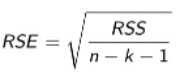
Residual Standard Error

average magnitude of unexplained variation remaining after fitting model

To practically measure prediction accuracy, we rely on the squared residuals summarized through the Residual standard Error (RSE).

Smaller RSE indicates predictions are closer to observed values.

Why is residual diagnostic important?

Residuals (ei = yi−ˆyi) capture the part of the dependent variable’s variation that the deterministic component of the model fails to explain, and therefore falls into the error term. If the model is well designed and accurately estimated, residuals should look like random noise. Checking them tells us whether the Gauss–Markov assumptions hold; if they are violated, our standard errors, p-values and CIs can be wrong.

Diagnostic issues: Heteroskedasticity, Autocorrelation, Non-normality / outliers , Non-linearity / omitted variables

Prediction errors

after fitting the model, part of the variation in Y remains unexplained, causing predicted values to differ from observed values

Statistical Model Building Framework

Pre-Modeling Phase:

o   Model specification

o   Data preparation

o   Data exploration

 

Modeling Phase:

o   Define estimation method

o   Estimate model coefficients

o   Check whether assumptions hold

 

Post Modeling (Diagnostic Phase):

o   Models fit & explanatory power

o   Residual diagnostic tests

o   Assess robustness & visual diagnostics

Causality

o   Not only established by correlation alone

o   Requires theory, identification strategies, research design that isolate effect of X on Y

o   Direction of relationship matters: if X → Y ; Y → X ; or X and Y both interact simultaneously

 

→ Relationship Distortion: through hidden factors (confounders Z → X ; Z → Y)

→ Artificial relationships: created through incorrect control for colliders (X → Z ←Y)

Model structure

Dependent variable (Y): the outcome to be explained

Independent variable(s) (X): the explanatory factors

Population

The complete set of all units of interest

Sample

The observed subset drawn from the population

Parameter

A fixed, usually unknown numerical feature of the population (µ, σ, π)

Statistics

A quantity computed from the sample (x, s, p); it estimates the parameter and varies from sample to sample

parameters describe populations; statistics describe samples. We use a statistic to estimate a parameter (unknown).

Explain how the following concepts build the foundation of statistics: Population → Sample → Distribution

• Population: The entire group we want to study.

• Sample: A subset of the population used to collect data.

• Distribution: Shows how the sample data are spread (e.g., mean, variance, shape), allowing us to infer characteristics of the population.

Key idea: We collect a sample from a population, analyze its distribution, and make conclusions about the population.

Why are data preparation and visualisation essential in empirical analysis, and how can weaknesses in these steps distort or bias the entire inference process?

• Data preparation ensures data are clean, complete, and accurate (handling missing values, errors, outliers).

• Visualisation helps detect patterns, trends, outliers, and data problems.

• Poor preparation or misleading visualisations can introduce bias, distort results, and lead to incorrect conclusions.

Key idea: "Garbage in, garbage out"—poor data quality leads to poor inference.

How do visualisation and summary statistics contribute to model specification?

• Visualisation reveals relationships, trends, non-linearity, and outliers.

• Summary statistics (mean, median, variance, correlation) describe the main features of the data.

• Together, they help choose the appropriate statistical model and check model assumptions.

What is the role of the literature in guiding statistical modelling?

• Literature provides theory and evidence to identify relevant variables and relationships.

• It guides model selection, assumptions, and interpretation of results.

• It helps avoid omitted-variable bias and ensures the model is scientifically justified.