Stat Econ Module 2

Two numerical ways of describing data

1. Measures of Location

2. Measures of Dispersion

Measures of Location (Central Tendency)

Pinpoint the center of a set of values.

Considering only measures of __________ can lead to erroneous conclusions; dispersion provides crucial additional context.

Measures of Dispersion (Variation/Spread)

Describe the spread or variability of the data.

Population

all the possible values or observations

Sample

a subset drawn from a population

Population Mean

The sum of all values divided by the number of values.

Population Mean Formula

μ = (ΣXᵢ) / N

where…

μ = __________

(ΣXᵢ) = sum of all X values in the population

N = number of values in the population

Parameter

any measurable characteristic of a population

ex: the mean of a population is an example of this

Parameter vs. Statistic

________ is any measurable characteristic of a population.

________ is any measurable characteristic of a sample.

Sample Mean Formula

x̄ = (ΣXᵢ) / n

where…

x̄ = ________

(ΣXᵢ) = sum of all x values in the sample

n = number of values in the sample

Statistic

Measure based on sample data

ex: mean of a sample

Properties of the Arithmetic Mean

• A mean exists for every set of interval or ratio-level data.

• Includes all values in computing the mean.

• A mean is unique for any given data set.

• The sum of deviations from the mean is always zero: Σ(X- x̄) = 0

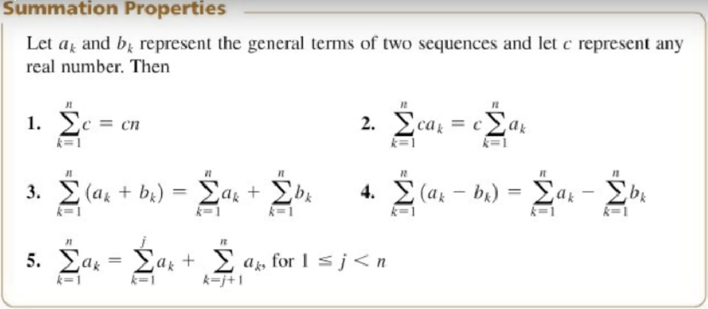
Summation Properties

Weakness of the Mean

Unduly affected by unusually large or small values (outliers), making it potentially unrepresentative.

Weighted Mean

Used when some values are more important than others. Each value is multiplied by its corresponding weight, summed, and then divided by the sum of the weights.

Ex: calculating for grades (where some are weighted more than others)

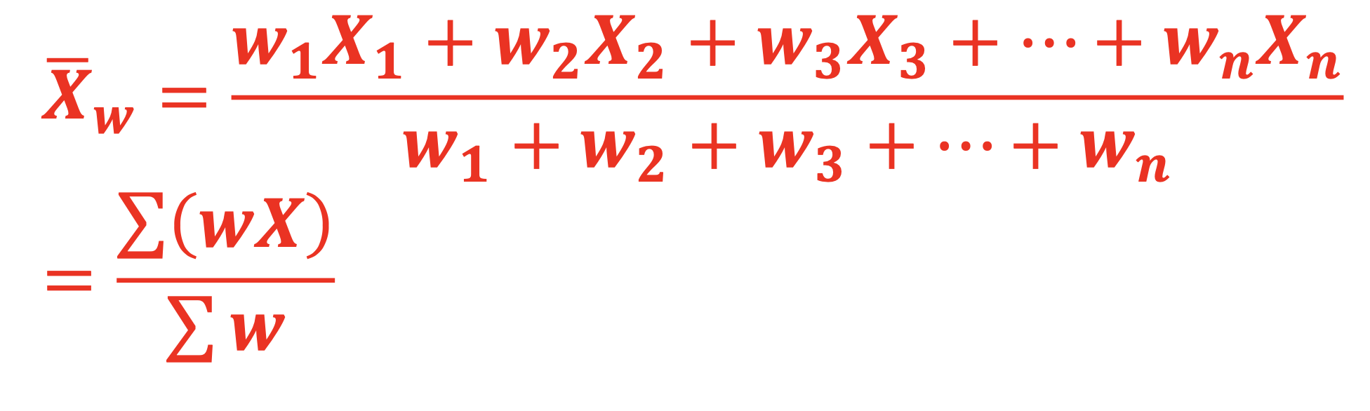
Weighted Mean Formula

(w₁x₁ + w₂x₂ + ... + wₙxₙ) / (w₁ + w₂ + ... + wₙ) = (Σwᵢxᵢ) / (Σwᵢ)

where…

the weight (w₁) of x₁ times x₁ plus the the weight (w₂) of x₂ times x₂… divided by the sum of the weights

Median

The midpoint of the values after they have been ordered from smallest to largest or largest to smallest.

Odd number of observations: The middle observation.

Even number of observations: The mean of the two middle observations. (May not be one of the original values).

Advantage: Unaffected by outliers

Mode

The value that appears most frequently in a data set.

Disadvantages

• May not exist (no value appears more than once).

• May have multiple modes (bimodal, multimodal).

• Less frequently used than mean or median.

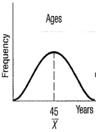
Mean = Median = Mode

for a symmetric mound-shape distribution

Skewed distribution

not symmetrical

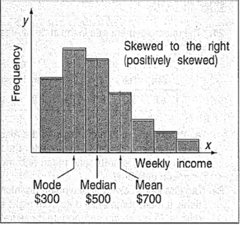
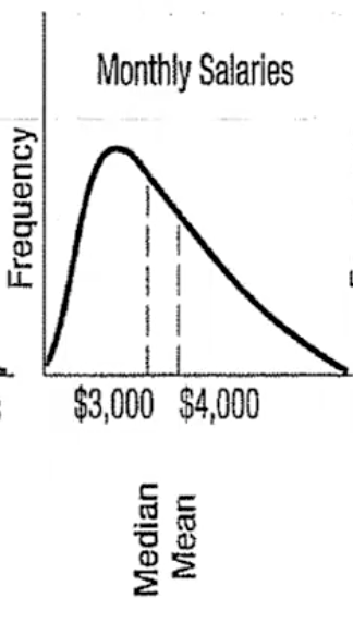
positively skewed distribution

a data distribution where most values are concentrated on the left side of the graph; skewed to the right (looks like a p)

the arithmetic mean is the largest of the three measures because the mean is influenced more than the median/mode by a few extremely high values

the median is the next largest measure in a ___________

mode is the smallest

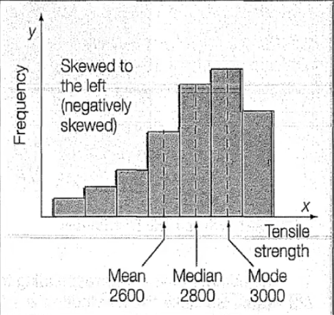
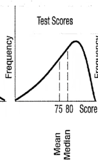
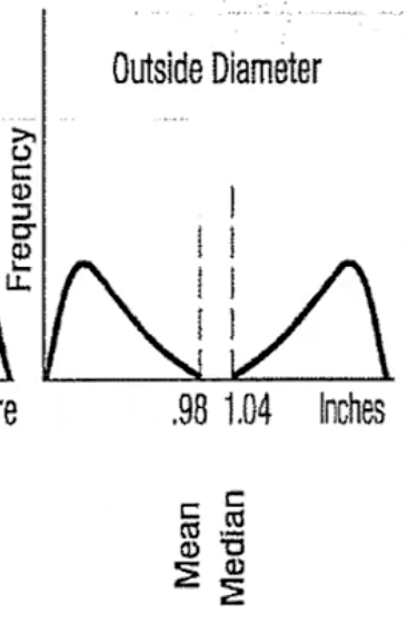
negatively skewed distribution

a data distribution where most values are concentrated on the right side of the graph (skewed to the left)

mean is the lowest of the three measures, influenced by a few extremely low observations

median is greater than mean

mode is the largest of the three

Mode is usually used for…

nominal-level data

Median is usually used for…

ordinal-level data

Mean is usually used for…

ratio-level data

Geometric Mean

useful for finding the average of percentages, ratios, indexes, or growth rates

ex: GDP which compound or build on each other

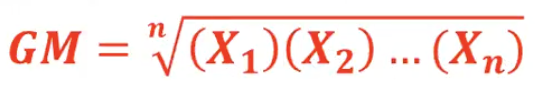
Geometric Mean Formula 1

n is the total number of terms (X) that are being multiplied

GM ≤ Arithmetic Mean

All data values must be positive

Geometric Mean vs. Arithmetic Mean

_________ uses addition and division to find the average of a set of numbers, while _________ uses multiplication and roots to find the average, particularly for growth rates or ratios.

The AM is suitable for additive data, while the GM is better for multiplicative relationships, such as investment returns or population growth, and requires positive numbers.

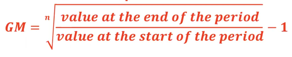
Geometric Mean Formula 2

to find an average percent increase over a period of time

ex: financial economics

Why study dispersion?

• Measures of location alone do not describe the spread of data.

• Allows for comparison of spread between two or more distributions.

ex: tour guide said river is avg. 3ft, but dispersion can say oh you can’t walk cuz there’s a 5 ft. section

Small Dispersion Meaning

data are clustered around the mean, making the mean representative.

Large Dispersion meaning

means the mean is less reliable as a representation of the data.

Range

Largest value - smallest value

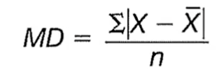
Mean Deviation

Measures the average distance of all the values from the mean.

The arithmetic mean of the absolute values of the deviations from the arithmetic mean.

x = the value of each observation

x̄ = arithmetic mean of the values

n = number of observations in the sample

| | = absolute value

Why absolute values in mean deviation

Without them, positive and negative deviations would cancel, resulting in a zero (useless) statistic.

Advantages of Mean Deviation

Uses all values, easy to understand.

Disadvantages of Mean Deviation

Use of absolute values makes it difficult to work with mathematically, less frequently used than standard deviation.

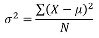
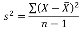
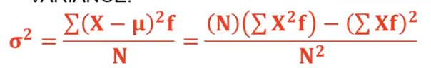
Variance

The arithmetic mean of the squared deviations from the mean.

• population variance (parameter)

• sample variance (statistic)

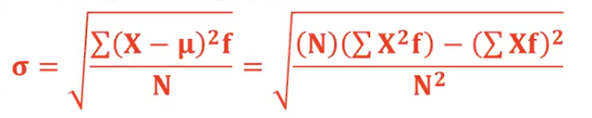
Standard Deviation

The square root of the variance. It is in the same units as the original data.

• Population Standard Deviation (parameter)

• Sample Standard Deviation (statistic)

Population Variance Formula

𝝈𝟐 = σ(𝑿 − 𝝁)𝟐 / 𝑵

Small variance means

populations whose values are near the mean

large variance means

population whose values are dispersed from the mean

Advantages of the variance

Uses all values, squaring deviations prevents cancellation (like absolute values but mathematically preferred). Always non-negative.

Disadvantages of the variance

Units are squared, making it difficult to interpret directly.

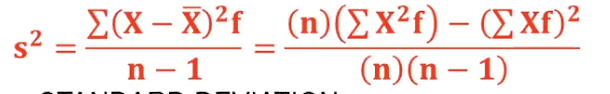
Sample Variance Formula

𝒔𝟐 = σ(𝑿 − ഥ𝑿)𝟐 / (𝒏 − 𝟏)

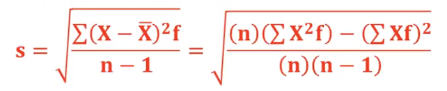
Sample standard deviation formula

𝒔 = √[σ(𝑿 − ഥ𝑿)𝟐 / (𝒏 − 𝟏)]

Interpretation and Uses of Standard Deviation

Commonly used to compare the spread in two or more sets of observations.

Ex: high standard deviation in index 500 funds means it’s makulit to show high risk and lower returns

low standard deviation means it’s safe and smaller, but less risky returns

Chebyshev's Theorem

determines the minimum proportion of the values that lie within a specified number of standard deviations of the mean

For any data set (any shape), the proportion of values within k standard deviations of the mean is at least 1 - (1/k²), where k is any constant greater than 1

Ex: 2 standard deviations away (plug it in to formula), means 75% of values lie 2 standard deviations away

Empirical Rule (Normal Rule)

For a symmetrical, bell-shaped distribution:

• Approximately 68% of observations are within ±1 standard deviation of the mean.

• Approximately 95% of observations are within ±2 standard deviations of the mean.

• Practically all (99.7%) observations are within ±3 standard deviations of the mean.

Population Standard Deviation

𝝈 = √[σ(𝑿 − 𝝁)𝟐 / 𝑵]

why use n-1

the denominator provides the appropriate correction" because using 'n' "tends to underestimate the population variance.

why discuss caculation of statistical descriptions from grouped data?

published data are often available in the form of a frequency distribution (ungrouped data is hard to get sometimes)

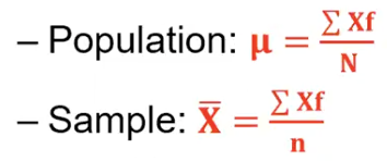
Mean of Grouped Data

Population: 𝝁 = (∑𝑿𝐟)/N

Sample: x̄ = (∑𝑿𝐟)/n

∑𝑿𝐟 is the sum of the products obtained by multiplying each class mark by the corresponding class frequency

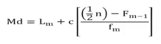
Median for Grouped Data

Md = median for grouped data

Lm = lower class boundary of the median class

c = class interval or class width

n = sample size

Fm-1 = cumulative of interval immediately preceding the median class

fm = frequency of the median class

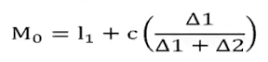
Mode for Grouped Data

M₀ = mode for grouped data

l₁ = lower class limit of the modal class

Δ1 = difference between the frequency of the modal class and the frequency of the preceding class (ignore the sign and just take the absolute value).

Δ2 = difference between the frequency of the model class and the frequency of the succeeding class (ignore the sign and just take the absolute value).

c = class interval or class width

Grouped Data Population Variance Formula

Grouped Data Population Standard Deviation Formula

Grouped Data Sample Variance Formula

Grouped Data Sample Standard Deviation Formula

To get from “ungrouped” to “grouped”…

substitute ∑𝑿 by ∑𝑿𝐟 and ∑𝑿² by ∑𝑿²𝐟

Box Plot

chart that is a graphical display, based on quartiles, that helps us picture a set of data

Statistics needed for a box plot

1. minimum value

2. first quartile

3. median

4. third quartile

5. maximum value

Outlier

• value that is inconsistent with the rest of the data, you need raw data

Outlier > Q₃ + 1.5(Q₃ - Q₁)

Outlier < Q₃ -1.5(Q₃ - Q₁)

skewness

lack of symmetry in a set of values

Symmetric

mean = median

• data values evenly spread around these values

• data values below mean and median are mirror image of those above 

Positively Skewed

set of values is skewed to the right if there is a single peak and the values extend much further to the right of the peak than to the left

• mean > median

Negatively skewed

there is a single peak, but the observation extend further to the left than to the right

• mean < median

Bimodal

two or more peaks

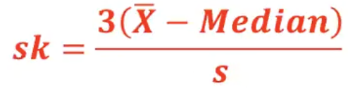
Pearson’s Coefficient of Skewness

based on the difference between the mean and median

• ranges from -3 to 3

value near -3 (Pearson)

considerable negative skewness

ex: -2.57

value near 3 (Pearson)

considerable positive skewness

value of 0 (Pearson)

mean = median

no skewness, symmetrical

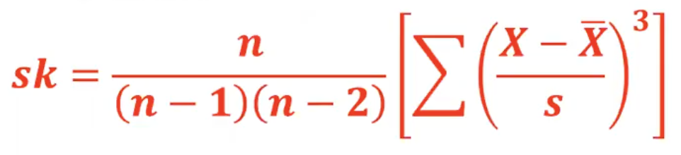
Software Coefficient of Skewness

shows the difference between each value and the mean, divided by standard deviation

• if difference is (+), the particular value is larger than the mean

• if difference is (-), is it smaller than the mean

• when cubed, it shows the information on the direction of the difference

Standardization

reports the difference between each value and the mean in units of the standard deviation

symmetric (Software Coefficient)

if standardized values are cubed and sum of lal the values would result to NEAR ZERO

positive skewness (Software Coefficient)

if there are several large values, clearly separate from the others, the sum of the cubed differences would be a LARGE POSITIVE VALUE

negative skewness (Software Coefficient)

several values much smaller will result in a NEGATIVE CUBED SUM

Unvariate Data

techniques to summarize the distribution of a single variable

Bivariate Data

two variables are measured for each individual or observation in the population or sample

• used often by data analysts

Scatter Diagram

graphical technique to show the relationship between variables

• variables in the x and y axis

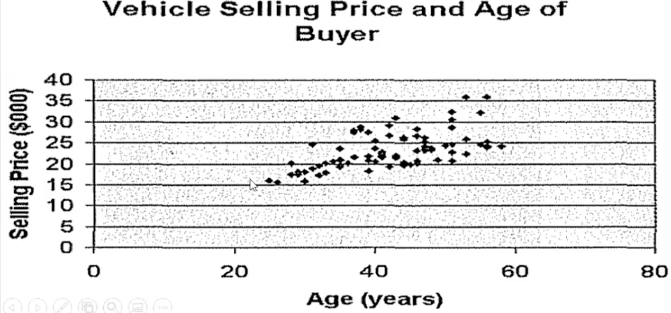
Positively Related (Scatter Diagram)

points move from lower left to upper right

Negatively Related (Scatter Diagram)

from upper left to lower right

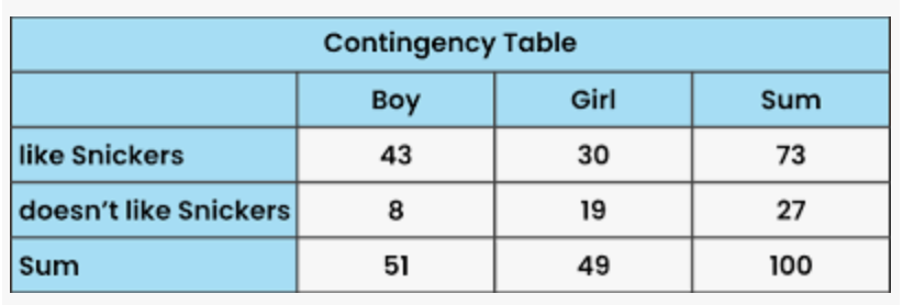
Contingency Table

table used to classify observations according to two identifiable characteristics

• for studying the relationship between two variables when one or both are nominal or ordinal scale