Paper 4: Further Probability and Statistics
 Call Kai
 Learn
Learn Practice Test
 Spaced Repetition
 Match
Match Flashcards
 Knowt Play
1/46

There's no tags or description
Looks like no tags are added yet.
Name | Mastery | Learn | Test | Matching | Spaced | Call with Kai | Chat |
|---|
No analytics yet
Send a link to your students to track their progress
47 Terms
Probability density function
A probability density function describes the probability of a continuous random variable falling within a particular interval of values, with the area between the function and the x-axis defining the probability over an interval and the y-axis being the probability density.
The probability over an interval therefore can be found by integrating the probability density function using the limits of the interval.
Since probability cannot take a negative value, the function cannot be negative or go below the x-axis.
Since the total probability for a continuous random variable is 1, the total area under the curve must be equal to 1.
Since the probability of a continuous random variable taking a single value is 0 (P(X = a) = 0), P(X < a) and P(X ≤ a) have the same value.
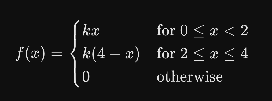
Probability density functions can be represented by a combination of different functions, each corresponding to part of the domain. These are known as piecewise probability density functions:
Cumulative distribution function
A cumulative distribution function calculates the accumulated probability of a continuous random variable taking a value less than or equal to a specific value of x.
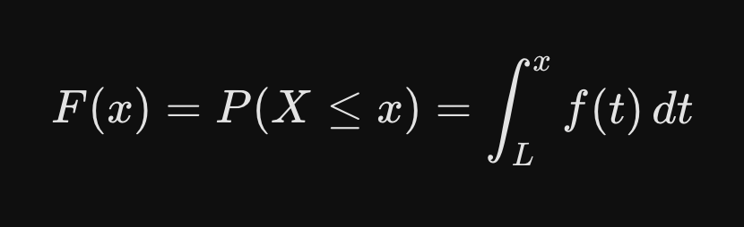
The cumulative distribution function is obtained by integrating each part of the piecewise probability density function using the lowest value of the domain (L) as the lower limit and x as the upper limit, adding the cumulative probability of the previous parts to the next part. A dummy variable (t) is used for the integration. The cumulative distribution function is also defined piecewise.
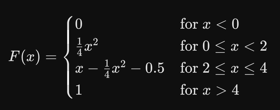
The cumulative distribution function can be used to directly find P(X ≤ x).
Obtaining a probability density function (f(x)) from a cumulative distribution function (F(x))
Differentiate each part of the piecewise cumulative distribution function, then define each part: f(x) = d/dx(F(x))
For parts of the cumulative distribution function that differentiate to 0, define the probability density function as 0 for ‘otherwise’.
Percentiles
The nth percentile of a continuous random variable, X, is the value of x where P(X ≤ x) = n/100.
The median is the 50th percentile, the lower quartile is the 25th percentile, and the upper quartile is the 75th percentile.
To find the nth percentile (x) from a cumulative distribution function, identify the correct interval of the piecewise cumulative distribution function, and set up the equation F(x) = n/100, then rearrange to find x.
To find the nth percentile from a probability distribution function, find the cumulative distribution function first.
Mode of a continuous random variable
The mode of a continuous random variable is the point with highest y-value (probability density) of a probability density function.
This is either at one of the end-points of the piecewise domains or at a maximum point.
Differentiate the probability density function, and compare with the y-values obtained from the end-points of the piecewise domains to find the highest.
Calculating E(X) of a continuous random variable X
Where f(x) is the probability density function of the continuous random variable X:
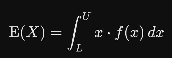
For continuous random variables defined with a piecewise probability density function, integrate each part of the function with their respective intervals as the limits then add them together.
Calculating E(g(X)) of a continuous random variable X
Where f(x) is the probability density function of the continuous random variable X, and g(X) is a function of X:
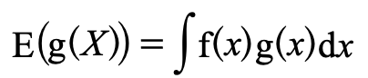
For continuous random variables defined with a piecewise probability density function, integrate each part of the function with their respective intervals as the limits, adding them together.
Calculating Var(X) of a continuous random variable X
Var(X) = E(X2) - (E(X))2
Consider the continuous random variable X with the cumulative distribution function
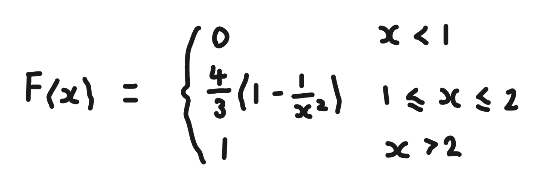
Find the cumulative distribution function of Y = X2 / 4
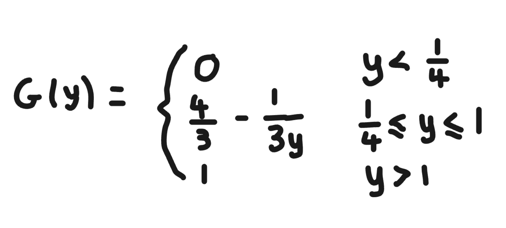
Define G(y), the cumulative distribution function of y:
G(y) = P(Y ≤ y)
Substitute the definition of Y: G(y) = P(X2 / 4 ≤ y)
Rearrange to make X the subject: G(y) = P(X ≤ 2√y)
G(y) = F(2√y)
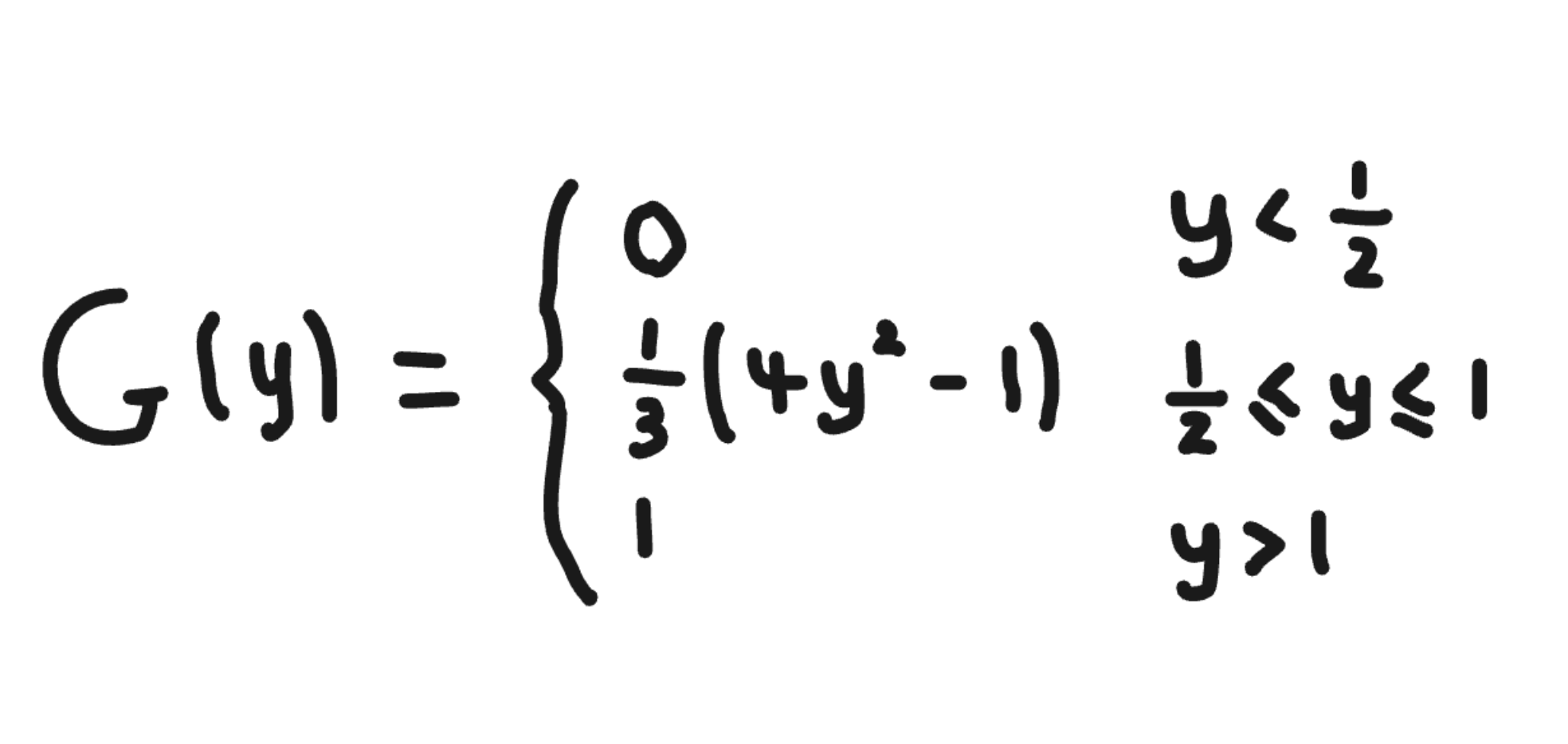
Form G(y) by substituting each x of F(x) with 2√y and transforming the intervals using Y = X2 / 4:
Consider the continuous random variable X with the cumulative distribution function
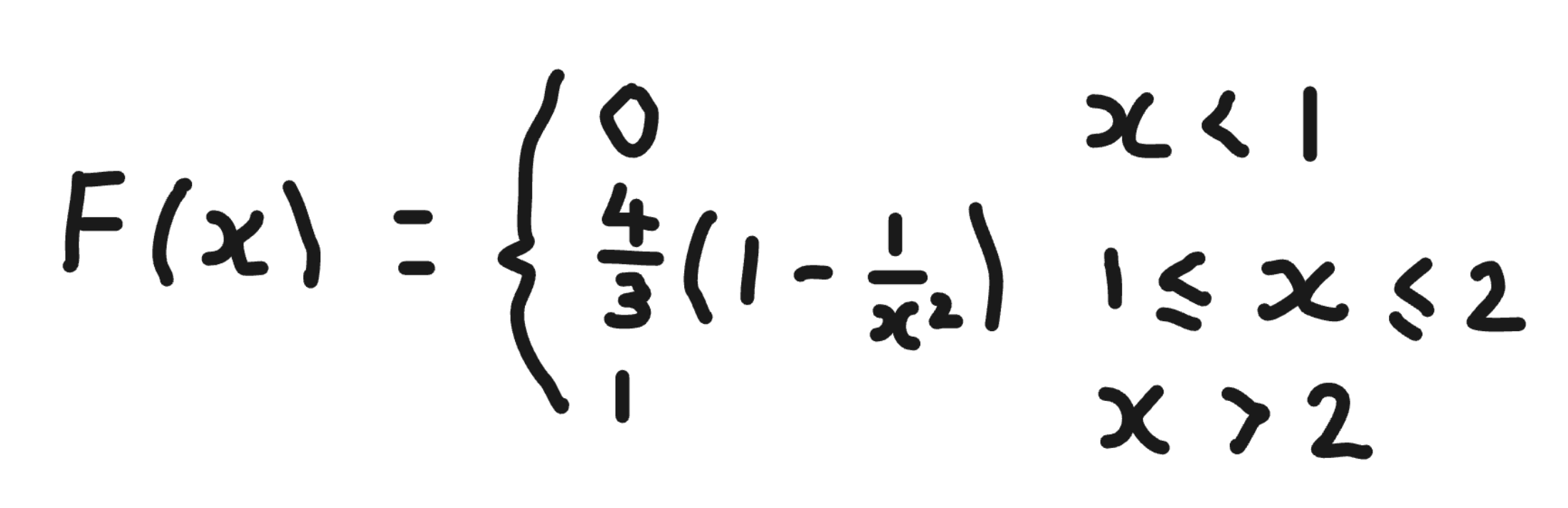
Find the cumulative distribution function of Y = 1/X
Define G(y), the cumulative distribution function of y:
G(y) = P(Y ≤ y)
Substitute the definition of Y: G(y) = P(1/X ≤ y)
Rearrange to make X the subject: G(y) = P(X ≥ 1/y)
G(y) = 1 - F(1/y)
Form line 2 of G(y): substitute x with 1/y in the middle formula of F(x) and subtract the result from 1. Transform the domain boundaries using Y = 1/X.
Form line 1 of G(y): if y < 1/2, then X ≥ 1/y where 1/y > 2. Since X cannot be greater than 2, P(Y ≤ y) = 0 for all y < 1/2.
Form line 3 of G(y): if y > 1, then X ≥ 1/y where 1/y < 1. Since X is always greater or equal to 1, P(Y ≤ y) = 1 for all y > 1.
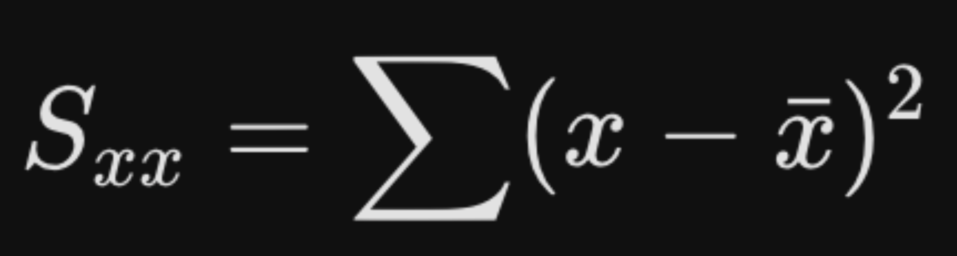
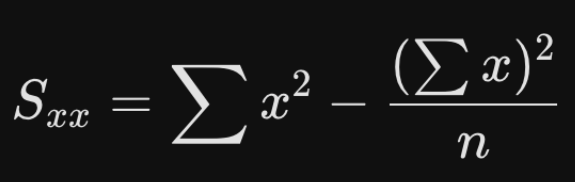
Sxx
Sum of squared deviations of x from its mean:
Degrees of freedom
The degrees of freedom of a calculation is the number of values in the calculation that are free to vary and are independent.
Degrees of freedom = n - number of parameters estimated
n = sample size
Unbiased estimator of the variance
A population’s variance can be estimated by taking a random sample from it and calculating the unbiased estimator of the variance, s2:
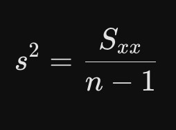
To ensure the estimator is unbiased, the formula involves division by the number of degrees of freedom (n - 1), as one parameter (the population mean, μ) has been estimated using the sample mean, x̄.
t-distribution curve
The t-distribution is a family of curves showing the probability distribution of the test statistic.
The y-axis is the probability density, and the x-axis is the test statistic.
Features of the curves include the following:
Mean = median = mode = 0, meaning the curve is centred at a test statistic of 0.
It is bell-shaped.
The total area beneath each curve is equal to 1.
It is symmetrical about the mean, which is at the centre peak.
The tails of the curve are asymptotic towards the x-axis.
The curves in the family vary in structure due to their varying degrees of freedom:
When the sample size and degrees of freedom are small, there is higher probability density at the tails.
When the sample size and degrees of freedom are large, there is less probability density at the tails.
When the degrees of freedom approaches infinity, the curve converges to the shape of the normal distribution curve.
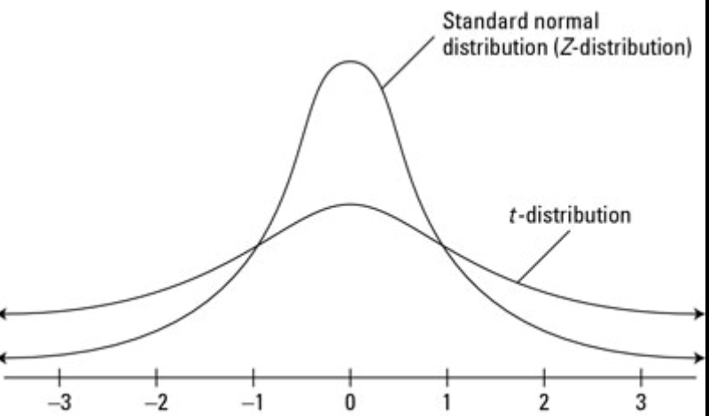
One-tailed and two-tailed tests
A one-tailed test tests whether the sample mean has a directional increase or decrease.
Right-tailed test: μ > k
Left-tailed test: μ < k
A two-tailed test tests whether the sample mean has an non-directional difference.
Critical value
The critical value is the boundary between the region of acceptance and rejection on a probability distribution: if the calculated test statistic is more extreme than the critical value, the null hypothesis H0 is rejected.
Significance level
The significance level is the area at the extremities of the curve that are rejected.
Single-sample t-test
A single-sample t-test is a hypothesis test that determines whether there is a significant difference between the mean of the sample group and the hypothesised mean of the population.
It is used when the population is normally distributed and when the population variance, σ2, is unknown.
State whether the test is a one-tailed or two-tailed test.
Two hypotheses are made:
Null hypothesis, H0: μ = k, where k is the assumed value of the mean that is being tested.
Assumes that any difference between the mean of the sample group and the hypothesised mean of the population has negligible meaning and is due to random sampling fluctuation.
Alternative hypothesis, H1: μ ≠ k / μ > k / μ < k, where k is the assumed value of the mean that is being tested.
A one-tailed test uses μ > k / μ < k.
A two-tailed test uses μ ≠ k.
Assumes the mean of the sample group and the hypothesised mean of the population have a statistically significant difference.
The test statistic / t-value is calculated: test statistic = (x̄ - μ) / (s / √n), where x̄ is the sample mean, s is the unbiased estimator of the standard deviation, μ is the hypothesised mean of the population, and n is the sample size.
The test statistic shows the number of standard errors the sample mean is away from the hypothesised mean of the population.
The numerator calculates the difference of the sample mean from the hypothesised mean of the population.
The denominator is the standard error of the mean. A high standard error of the mean indicates that the sample mean is unstable and is unreliable as a representation of the population mean. A low standard error of the mean indicates that the sample mean is stable and is a reliable representation of the population mean.
The critical value is found:
Critical value = tp, n-1
One-tailed test: p = 1 - significance level
Two-tailed test: p = 1 - (significance level / 2)
n-1 is the degree of freedom.
The critical value is found by using a t-distribution table and locating the value of p and the degrees of freedom. We make the critical value positive for a right-tailed test, negative for a left-tailed test, or matching the sign of the test statistic for a two-tailed test.
The null hypothesis H0 is then not rejected if the calculated test statistic is less extreme than the critical value and is rejected if the calculated test statistic is more extreme than the critical value.
The conclusion is stated:
If H0 is not rejected: ‘there is insufficient evidence to suggest [H1]’, where H1 is written in the context of the question.
If H0 is rejected: ‘there is sufficient evidence to suggest [H1]’, where H1 is written in the context of the question.
2-sample Z-test
A 2-sample Z-test is a hypothesis test that determines if there is a significant difference from the hypothesised difference of two population means.
It is used when the true population variances are known, the true population variances are unknown for n ≥ 30, the two groups of data are independent from each other, and the populations are normally distributed.
State whether the test is a one-tailed or two-tailed test.
Two hypotheses are made:
Null hypothesis, H0: μ1 - μ2 = k
Assumes that any difference from the hypothesised difference of the two population means has negligible meaning and is due to random sampling fluctuation.
Alternative hypothesis, H1: μ1 - μ2 ≠ k / μ1 - μ2 > k / μ1 - μ2 < k
One-tailed test: μ1 - μ2 > k / μ1 - μ2 < k
Two-tailed test: μ1 - μ2 ≠ k
Assumes that any difference from the hypothesised difference of the two population means is statistically significant.
The test statistic / z-value is calculated, where x̄ is the sample mean, μ is the hypothesised mean of the population, σ2 is the population variance, and n is the sample size:
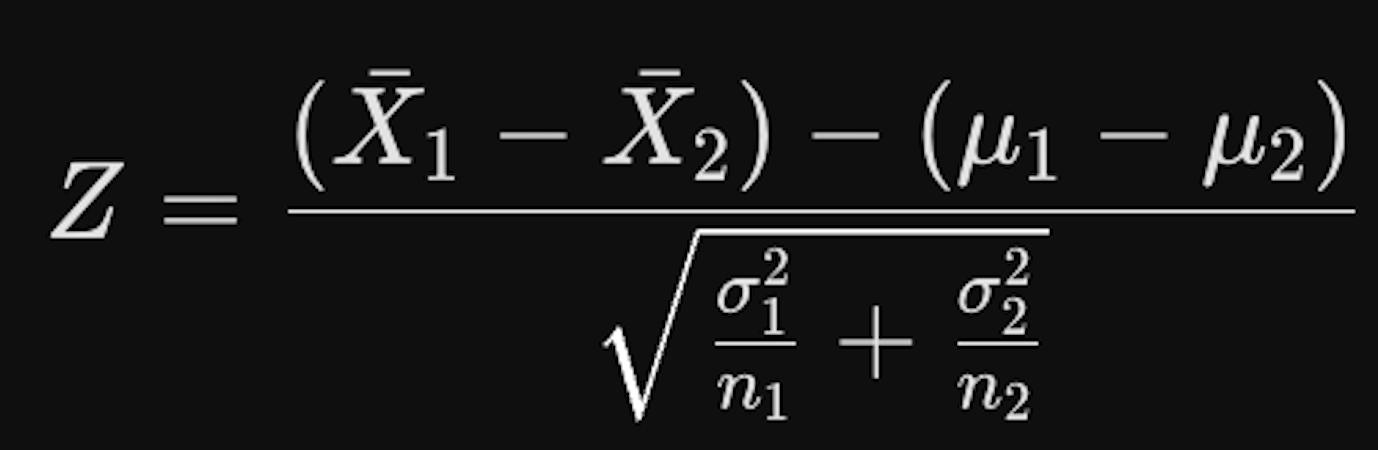
If the population variances are unknown, the unbiased estimator of the variances is used.
The test statistic shows how many standard errors the difference in sample means is away from the hypothesised difference.
The numerator calculates the difference between the difference of the two sample means and the hypothesised difference between the population means.
The denominator is the standard error of the difference between means. A high standard error indicates that the calculated difference is sample means is unstable and unreliable as a representation of the difference between population means. A low standard error indicates that the difference between the sample means is stable and a reliable representation of the difference between population means.
The critical value is found using the normal distribution table:
Find the area of rejection in each tail, which is equal to the significance level for a one-tailed test and is equal to the significance level / 2 for a two-tailed test.
1 - area of rejection = target area, which is located in the table body to find the critical value.
We make the critical value positive for a right-tailed test, negative for a left-tailed test, or matching the sign of the test statistic for a two-tailed test.
The null hypothesis H0 is then not rejected if the calculated test statistic is less extreme than the critical value and is rejected if the calculated test statistic is more extreme than the critical value.
The conclusion is stated:
If H0 is not rejected: ‘there is insufficient evidence to suggest [H1]’, where H1 is written in the context of the question.
If H0 is rejected: ‘there is sufficient evidence to suggest [H1]’, where H1 is written in the context of the question.
Pooled estimator of common variance
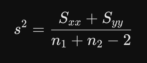
A pooled estimator of a common variance is used when two populations have unknown but equal variances to estimate this variance.
When you are not given unbiased estimators of the variance for each sample, the following formula is used:
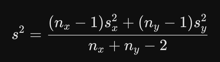
When you are given the unbiased estimators of the variance for each sample, the following formula can be derived from the previous:
2-sample t-test
A 2-sample t-test is a hypothesis test that determines if there is a significant difference from the hypothesised difference of two population means.
It is used when the two groups of data are independent from each other, are normally distributed, and the true variances of the populations are unknown but the same.
Sample sizes can be small.
State whether the test is a one-tailed or two-tailed test.
Two hypotheses are made:
Null hypothesis (H0): μ1 - μ2 = k
Assumes that any difference from the hypothesised difference of the two population means has negligible meaning and is due to random sampling fluctuation.
Alternative hypothesis (H1): μ1 - μ2 ≠ k, μ1 - μ2 > k, μ1 - μ2 < k
A one-tailed test uses μ1 - μ2 > k / μ1 - μ2 < k
A two-tailed test uses μ1 - μ2 ≠ k
Assumes that any difference from the hypothesised difference of the two population means is statistically significant.
The pooled estimator of the common variance is calculated.
The test statistic / t-value is calculated, where x̄ is the sample mean, μ is the hypothesised mean of the population, s2 is the pooled estimator of common variance, and n is the sample size:
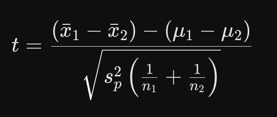
The test statistic shows how many standard errors the difference in sample means is away from the hypothesised difference.
The numerator calculates the difference between the difference of the two sample means and the hypothesised difference between the population means.
The denominator is the standard error of the difference between means. A high standard error indicates that the calculated difference in sample means is unstable and unreliable as a representation of the difference between population means. A low standard error indicates that the difference between the sample means is stable and a reliable representation of the difference between population means.
The critical value is found:
Critical value = tp, n1 + n2 -2
One-tailed test: p = 1 - significance level
Two-tailed test: p = 1 - (significance level / 2)
n1 + n2 - 2 is the degree of freedom.
The critical value is found by using a t-distribution table and locating the value of p and the degrees of freedom. We make the critical value positive for a right-tailed test, negative for a left-tailed test, or matching the sign of the test statistic for a two-tailed test.
The null hypothesis H0 is then not rejected if the calculated test statistic is less extreme than the critical value and is rejected if the calculated test statistic is more extreme than the critical value.
The conclusion is stated:
If H0 is not rejected: ‘there is insufficient evidence to suggest [H1]’, where H1 is written in the context of the question.
If H0 is rejected: ‘there is sufficient evidence to suggest [H1]’, where H1 is written in the context of the question.
Paired sample t-test
A paired sample t-test is used to measure the effect of a variable on a set of data that is measured twice: before the change in variable and after. The mean of the differences between each pair of data is calculated.
It is used when the two groups of data contain corresponding pairs and the population of differences between the pairs of data are normally distributed.
State whether the test is a one-tailed or two-tailed test.
Two hypotheses are made:
Null hypothesis, H0: μd = k
Assumes that any mean difference observed between the paired measurements that is different to the hypothesised mean difference has negligible meaning and is due to random sampling fluctuation.
Alternative hypothesis, H1: μd ≠ k, μd > k, μd < k
Right-tailed test: μd > k
Left-tailed test: μd < k
Two-tailed test: μd ≠ k
Assumes that any mean difference observed between the paired measurements that is different from the hypothesised mean difference is statistically significant.
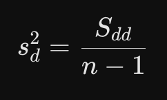
Calculate the unbiased estimator of the variance of the differences, where n is the number of data pairs:
The test statistic / t-value is calculated, where d̄ is the sample mean difference between the pairs of data, μd is the hypothesised mean difference between the pairs of data, s2d is the unbiased estimator of the variance of the differences, and n is the number of data pairs:
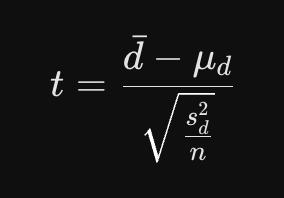
The test statistic shows how many standard errors the sample’s mean of the differences between the pairs of data is away from the hypothesised mean of the differences.
The numerator is the sample mean of the differences between the pairs of data.
The denominator is the standard error of the mean difference. A high standard error indicates that the calculated mean of the differences between the pairs of data is unstable and unreliable as a representation of the mean difference present in the population. A low standard error indicates that the calculated mean of the differences between the pairs of data is stable and a reliable representation of the mean difference present in the population.
The critical value is found:
Critical value = tp, n-1
One-tailed test: p = 1 - significance level
Two-tailed test: p = 1 - (significance level / 2)
n-1 is the degree of freedom.
The critical value is found by using a t-distribution table and locating the value of p and the degrees of freedom. We make the critical value positive for a right-tailed test, negative for a left-tailed test, or matching the sign of the test statistic for a two-tailed test.
The null hypothesis H0 is then not rejected if the calculated test statistic is less extreme than the critical value and is rejected if the calculated test statistic is more extreme than the critical value.
The conclusion is stated:
If H0 is not rejected: ‘there is insufficient evidence to suggest [H1]’, where H1 is written in the context of the question.
If H0 is rejected: ‘there is sufficient evidence to suggest [H1]’, where H1 is written in the context of the question.
Confidence interval for a population mean using the t-distribution
The confidence interval for a population mean is a range of values that is likely to contain the true population mean (μ) at a specified confidence percentage. For example, a 95% confidence interval means that if samples were taken many times and a 95% confidence interval was calculated each time, 95% of the intervals would include the true population mean (μ).
When the population variance is unknown, the t-distribution is used.
Confidence interval = x̄ ± (tp, n-1)(s/√n), where x̄ is the sample mean, tp, n-1 is the critical value for a two-tailed test, s is the unbiased estimator of the standard deviation, and n is the sample size.
The confidence interval is written in the form [lower bound, upper bound]
Confidence interval + significance level = 100%
Confidence interval for a difference in population means using the normal distribution
The confidence interval for a difference in population means is a range of values that is likely to contain the true difference in population means at a specified confidence percentage. For example, a 95% confidence interval means that if samples were taken many times and a 95% confidence interval was calculated each time, 95% of the intervals would include the true difference in population means.
When the population variances are known or when they are unknown and n ≥ 30, the normal distribution is used.
To find the confidence interval, the following formula is used, where x̄ and ȳ are the sample means, the critical value is for a two-tailed test, σ2 is the variance, and nx and ny are the sample sizes:

The confidence interval is written in the form [lower bound, upper bound]
Confidence interval + significance level = 100%
Confidence interval for a difference in population means using the t-distribution
The confidence interval for a difference in population means is a range of values that is likely to contain the true difference in population means at a specified confidence percentage. For example, a 95% confidence interval means that if samples were taken many times and a 95% confidence interval was calculated each time, 95% of the intervals would include the true difference in population means.
When the population variances are unknown but assumed equal, the t-distribution is used.
To find the confidence interval, the following formula is used, where x̄ and ȳ are the sample means, tp, nx + ny - 2 is the critical value for a two-tailed test, s2p is the pooled estimator of the common variance, and nx and ny are the sample sizes:

The confidence interval is written in the form [lower bound, upper bound]
Confidence interval + significance level = 100%
Poisson distribution
The Poisson distribution is a discrete probability distribution that models the number of times an event occurs in a fixed interval of time, e.g. the number of particles emitted by a radioactive source per second.
For a probability distribution to be a Poisson distribution, the following criteria must be met:
Events are discrete
Events are independent
The average number of events per unit of time (λ) remains constant.
E(x) = Var(X) = λ
A discrete random variable, X, that has a Poisson distribution is denoted by X ~ Po (λ), where λ is the average number events per unit of time.
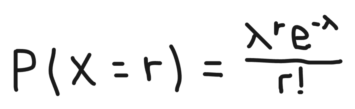
The probability of observing r events in an interval is found using the following formula, where X is the discrete random variable representing the number of events in an interval, and λ is the average number of events per interval:
Discrete uniform distribution
A discrete probability distribution in which the random variable takes specific values, and each value has an equal probability.
Continuous uniform distribution
A continuous probability distribution in which the random variable takes any real value within an interval, and there is a constant probability density across that interval.
A continuous random variable, X, that has a uniform distribution is denoted by X ~ U(a,b), where a is the lower bound of the interval and b is the upper bound of the interval.
The following is the probability density function for a continuous uniform distribution, where a is the lower bound of the interval and b is the upper bound of the interval:

χ2-distribution curve
The χ2-distribution is a family of curves showing the probability distribution of the test statistic.
The y-axis is the probability density, and the x-axis is the test statistic.
Features of the curves include the following:
Test statistic ≥ 0
It is non-symmetrical and right-skewed.
The total area beneath the curve is equal to 1.
The left tail starts sharply at the origin, and the right tail is asymptotic to the positive x-axis.
The curves in the family vary in structure due to their varying degrees of freedom:
When the sample size and degrees of freedom increase, the curve’s peak moves to the right.

χ2 goodness of fit test
A χ2 goodness of fit test is used to determine whether a given probability distribution matches a hypothesised distribution.
Possible hypothesised distributions include a discrete uniform distribution, a binomial distribution, a Poisson distribution, a continuous uniform distribution, and a normal distribution.
Two hypotheses are made:
Null hypothesis (H0): The [distribution] is a good-fit model for the data.
Alternative hypothesis (H1): The [distribution] is not a good-fit model for the data.
For the results of the χ2 goodness of fit test to be valid, the expected frequency of every category must be greater or equal to 5 (E ≥ 5).
If the expected frequency of a category is less than 5, frequencies of adjacent categories must be combined.
The expected frequency (E) of each category is calculated:
Discrete uniform distribution: E = total sample size / number of categories
Binomial distribution: E = ((nCr)(pr)(1-p)n-r)(total sample size)
Poisson distribution: E = ((λxe-λ)/x!)(total sample size)
Continuous uniform distribution: E = (class width)(probability density)(total sample size)
Normal distribution: E = (area under curve)(total sample size)
Ensure that the smallest interval includes all of the values below it in the lower tail and that the largest interval includes all of the values above it in the upper tail.
To find the probability of the final interval, use 1 - sum of previous intervals’ probabilities
The test statistic is calculated, where O is the observed frequency, E is the expected frequency, and Σ means that the result of each category are added together:
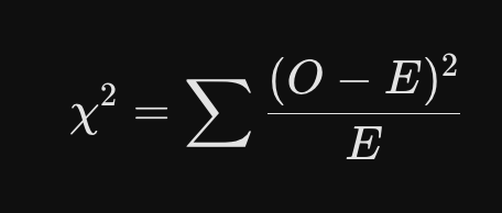
The degrees of freedom are calculated and stated: df = number of categories after combination - number of parameters estimated - 1
1 is subtracted because the frequency of the last category is fixed / predetermined to equal the total number of observations, so there is 1 fewer independent categories.
Discrete uniform distribution: 0 parameters estimated
Binomial distribution: 1 parameter estimated if p is calculated
Poisson distribution: 1 parameter estimated if λ is calculated
Continuous uniform distribution: 0 parameters estimated
Normal distribution: 2 parameters estimated if μ and σ2 are calculated
The critical value is found:

p = 1 - significance level
The critical value is found by using a χ2 distribution table and locating the values of p and the degrees of freedom.
The null hypothesis H0 is then not rejected if the calculated test statistic is less extreme than the critical value and is rejected if the calculated test statistic is more extreme than the critical value.
The conclusion is stated, adding context for the question:
If H0 is not rejected: ‘there is insufficient evidence to suggest [H1]’
If H0 is rejected: ‘there is sufficient evidence to suggest [H1]’
χ2 independence test
A χ2 independence test is used to determine whether there is a statistically significant association between two categorical variables.
A contingency table is used to organise frequency data across the two categorical variables.
Two hypotheses are made:
Null hypothesis (H0): There is no association between [Variable 1] and [Variable 2].
Alternative hypothesis (H1): There is an association between [Variable 1] and [Variable 2].
For the results of the χ2 independence test to be valid, the expected frequency of every cell of the contingency table must be greater or equal to 5 (E ≥ 5).
If the expected frequency of a cell is less than 5, frequencies of adjacent rows or columns must be combined.
The expected frequency (E) of each cell is calculated: (row total)(column total) / total sample size
Probability of a random selection being in a particular row = row total / total sample size
Probability of a random selection being in a particular column = column total / total sample size
If the row variable and column variable are independent, the probability of a random selection being in a particular row and a particular column = (row total / total sample size)(column total / total sample size)
Expected frequency (E) of a cell = (total sample size)(row total / total sample size)(column total / total sample size) = (row total)(column total) / total sample size
The test statistic is calculated, where O is the observed frequency, E is the expected frequency, and Σ means that the result of each cell are added together:

The degrees of freedom are calculated and stated: df = (number of rows - 1)(number of columns - 1)
In any individual row, the last cell is not free to vary.
In any individual column, the last cell is not free to vary.
Since these two restrictions occur simultaneously, the total degrees of freedom is equal to the product of the degrees of freedom of any individual row and any individual column.
The critical value is found:

p = 1 - significance level
The critical value is found by using a χ2 distribution table and locating the values of p and the degrees of freedom.
The null hypothesis H0 is then not rejected if the calculated test statistic is less extreme than the critical value and is rejected if the calculated test statistic is more extreme than the critical value.
The conclusion is stated:
If H0 is not rejected: ‘there is insufficient evidence to suggest [H1]’
If H0 is rejected: ‘there is sufficient evidence to suggest [H1]’
Non-parametric test
A non-parametric test is a hypothesis test that makes no assumptions about the underlying population distribution or its parameters.
It is used in the following situations:
When the population cannot be assumed to be normally distributed.
When the data has extreme outliers.
Single-sample sign test
A single-sample sign test is a non-parametric test used to determine if the median of a population equals a hypothesised value.
It is used when the data is continuous and independent from each other.
Two hypotheses are made:
Null hypothesis (H0): m = k
Alternative hypothesis (H1): m ≠ k / m > k / m < k
Two-tailed test: m ≠ k
One-tailed test: m > k / m < k
Mark each piece of data in the sample with a plus sign if it is greater than the hypothesised median and a minus sign if it is less.
The test statistic is equal to the number of plus signs.
The test statistic (X) follows the following binomial distribution because, under H0, each data value has a 0.5 probability of falling above or below the true population median:

When 0.5n ≤ 5, the probability of the test statistic is calculated using the binomial distribution:
Right-tailed test (m > k): P(X ≥ test statistic)
In a right-tailed test, we are looking for evidence that the median is greater than its hypothesised value, so we find the probability of obtaining that number of pluses or more if the median is as hypothesised. A low probability indicates the true median is greater than hypothesised.
Left-tailed test (m < k): P(X ≤ test statistic)
In a left-tailed test, we are looking for evidence that the median is less than its hypothesised value, so we find the probability of obtaining that number of pluses or less if the median is as hypothesised. A low probability indicates the true median is less than hypothesised.
Two-tailed test (m ≠ k): P(X ≤ test statistic) x 2 / P(X ≥ test statistic) x 2
In a two-tailed test, we are looking for evidence that the median differs from its hypothesised value, so we find the probability of obtaining that number of pluses or less/more if the median is as hypothesised. We identify which tail the number of pluses lies in and calculate the tail’s probability: if + > - then it is the right tail, and if + < - then it is the left tail. The probability obtained is multiplied by two to account for both tails. A low probability indicates that the true median is different to the hypothesised value.
When 0.5n > 5, the probability of the test statistic is calculated by approximating the binomial distribution using a normal distribution:
X ~ B(n, 0.5) can be approximated by X ~ N(μ,σ2), where μ = 0.5n and σ2 = 0.25n
A continuity correction of ±0.5 must be applied.
Right-tailed test (m > k):

Left-tailed test (m < k):

Two-tailed test (m ≠ k): we identify which tail the number of pluses lies in and calculate the tail’s probability and multiply by two.
H0 is rejected if the probability of the test statistic is less than the significance level and is not rejected if the probability of the test statistic is greater than the significance level.
A probability less than the significance level indicates that the test outcome is too improbable to have occurred by chance if the median were k.
A probability more than the significance level indicates that the test outcome is probable enough to have occurred by chance if the median were k.
The conclusion is stated:
If H0 is not rejected: ‘there is insufficient evidence to suggest [H1]’
If H0 is rejected: ‘there is sufficient evidence to suggest [H1]’
Single-sample Wilcoxon signed-rank test
A single-sample Wilcoxon signed-rank test is a non-parametric test used to determine if the median of a population equals a hypothesised value.
It is used when the data is continuous, independent from each other, and is symmetrical around the median.
Two hypotheses are made:
Null hypothesis (H0): m = k
Alternative hypothesis (H1): m ≠ k / m > k / m < k
Two-tailed test: m ≠ k
One-tailed test: m > k / m < k
For each data value, calculate the difference from the hypothesised median (d = x - k).
Rank the absolute differences in ascending order from 1 to n.
Calculate the sum of the positive difference ranks and then the sum of the negative difference ranks.
The test statistic is equal to the smallest of the two sums of ranks.
For n ≤ 20, the Wilcoxon signed-rank test table is used:
Right-tailed test (m > k): H0 is rejected if the test statistic is the negative rank sum and test statistic ≤ critical value.
In a right-tailed test, we are looking for evidence that the median is greater than the hypothesised value, requiring the negative rank sum to be less than the positive rank sum and, hence, the test statistic.
Left-tailed test (m < k): H0 is rejected if the test statistic is the positive rank sum and test statistic ≤ critical value.
In a left-tailed test, we are looking for evidence that the median is less than the hypothesised value, requiring the positive rank sum to be less than the negative rank sum and, hence, the test statistic.
Two-tailed test (m ≠ k): H0 is rejected if test statistic ≤ critical value
In a two-tailed test, we are looking for evidence that the median differs from the hypothesised value in either direction, so the test statistic can be either the positive rank sum or the negative rank sum.
For n > 20, the probability of the test statistic is calculated by approximating the distribution with a normal distribution:
The test statistic is X ~ N(μ,σ2), where μ = ¼ n(n+1) and σ2 = 1/24 n(n+1)(2n+1)
A continuity correction of +0.5 must be applied because the probability of the lower tail is found.
Right-tailed test (m > k): H0 is rejected if the test statistic is the negative rank sum and the lower tail probability of the test statistic is less than or equal to the significance level.

Left-tailed test (m < k): H0 is rejected if the test statistic is the positive rank sum and the lower tail probability of the test statistic is less than or equal to the significance level.
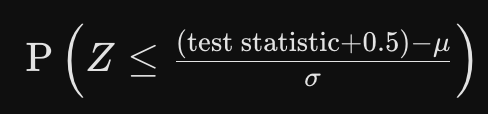
Two-tailed test (m ≠ k): H0 is rejected if the lower tail probability of the test statistic multiplied by two is less than or equal to the significance level.

The conclusion is stated:
If H0 is not rejected: ‘there is insufficient evidence to suggest [H1]’
If H0 is rejected: ‘there is sufficient evidence to suggest [H1]’
Paired-sample sign test
A paired-sample sign test is a non-parametric test used to determine if there is a significant difference between a pair of populations by testing whether the median difference equals 0.
It is used when the data are in matched pairs, the differences between the matched pairs are continuous, and the data pairs are independent from each other.
Two hypotheses are made:
Null hypothesis (H0): md = 0
Alternative hypothesis (H1): md ≠ 0 / md > 0 / md < 0
Right-tailed test: md > 0
Left-tailed test: md < 0
Two-tailed test: md ≠ 0
For each pair of data, the difference is calculated.
Positive differences are marked with a plus, and negative differences are marked with a minus.
The test statistic is equal to the number of plus signs.
The test statistic (X) follows the following binomial distribution because, under H0, each difference has a 0.5 probability of being less than zero or more than zero.
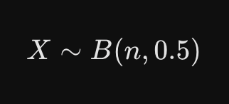
When 0.5n ≤ 5, the probability of the test statistic is calculated using the binomial distribution:
Right-tailed test (md > 0): P(X ≥ test statistic)
In a right-tailed test, we are looking for evidence that the median difference is greater than 0, so we find the probability of obtaining that number of pluses or more if the median difference is 0. A low probability indicates the true median difference is greater than 0.
Left-tailed test (md < 0): P(X ≤ test statistic)
In a left-tailed test, we are looking for evidence that the median difference is less than 0, so we find the probability of obtaining that number of pluses or less if the median difference is 0. A low probability indicates the true median difference is less than 0.
Two-tailed test (md ≠ 0): P(X ≤ test statistic) x 2 / P(X ≥ test statistic) x 2
In a two-tailed test, we are looking for evidence that the median difference differs from 0, so we find the probability of obtaining that number of pluses or less/more if the median difference is 0. We identify which tail the number of pluses lies in and calculate the tail’s probability: if + > - then it is the right tail, and if + < - then it is the left tail. The probability obtained is multiplied by two to account for both tails. A low probability indicates that the true median difference is different to 0.
When 0.5n > 5, the probability of the test statistic is calculated by approximating the binomial distribution with a normal distribution.
X ~ B(n, 0.5) can be approximated by X ~ N(μ,σ2), where μ = 0.5n and σ2 = 0.25n
A continuity correction of ±0.5 must be applied.
Right-tailed test (md > 0):
Left-tailed test (md < 0):
Two-tailed test (md ≠ 0): we identify which tail the number of pluses lies in and calculate the tail’s probability and multiply by two.
H0 is rejected if the probability of the test statistic is less than the significance level and is not rejected if the probability of the test statistic is greater than the significance level.
A probability less than the significance level indicates that the test outcome is too improbable to have occurred by chance if the median difference were 0.
A probability more than the significance level indicates that the test outcome is probable enough to have occurred by chance if the median difference were 0.
The conclusion is stated:
If H0 is not rejected: ‘there is insufficient evidence to suggest [H1]’
If H0 is rejected: ‘there is sufficient evidence to suggest [H1]’
Wilcoxon matched-pairs signed-rank test
A Wilcoxon matched-pairs signed-rank test is a non-parametric test used to determine if there is a significant difference between a pair of populations by testing whether the median difference equals 0.
It is used when the data are in matched pairs, the differences between the matched pairs are continuous and symmetrical around the median, and the data pairs are independent from each other.
Two hypotheses are made:
Null hypothesis (H0): md = 0
Alternative hypothesis (H1): md ≠ 0 / md > 0 / md < 0
Right-tailed test: md > 0
Left-tailed test: md < 0
Two-tailed test: md ≠ 0
For each pair of data, the difference is calculated.
Rank the absolute differences in ascending order from 1 to n. Add negative signs to the negative difference ranks.
Calculate the sum of the positive difference ranks (P) and then the sum of the negative difference ranks (Q).
The test statistic is equal to the smallest of the two sums of ranks.
For n ≤ 20, the Wilcoxon signed-rank test table is used:
Right-tailed test (md > 0): H0 is rejected if the test statistic is the negative rank sum and test statistic ≤ critical value.
In a right-tailed test, we are looking for evidence that the median difference is greater than 0, requiring the negative rank sum to be less than the positive rank sum and, hence, the test statistic.
Left-tailed test (md < 0): H0 is rejected if the test statistic is the positive rank sum and test statistic ≤ critical value.
In a left-tailed test, we are looking for evidence that the median difference is less than 0, requiring the positive rank sum to be less than the negative rank sum and, hence, the test statistic.
Two-tailed test (md ≠ 0): H0 is rejected if test statistic ≤ critical value
In a two-tailed test, we are looking for evidence that the median difference differs from 0 in either direction, so the test statistic can be either the positive rank sum or the negative rank sum.
For n > 20, the probability of the test statistic is calculated by approximating the distribution with a normal distribution:
The test statistic is X ~ N(μ,σ2), where μ = ¼ n(n+1) and σ2 = 1/24 n(n+1)(2n+1)
A continuity correction of +0.5 must be applied because the probability of the lower tail is found.
Right-tailed test (md > 0): H0 is rejected if the test statistic is the negative rank sum and the lower tail probability of the test statistic is less than or equal to the significance level.
Left-tailed test (md < 0): H0 is rejected if the test statistic is the positive rank sum and the lower tail probability of the test statistic is less than or equal to the significance level.
Two-tailed test (md ≠ 0): H0 is rejected if the lower tail probability of the test statistic multiplied by two is less than or equal to the significance level.
The conclusion is stated:
If H0 is not rejected: ‘there is insufficient evidence to suggest [H1]’
If H0 is rejected: ‘there is sufficient evidence to suggest [H1]’
Wilcoxon rank-sum test
A Wilcoxon rank-sum test is a non-parametric test used to determine if there is a significant difference between two populations by testing if they have the same median.
It is used when the data consists of two samples of sizes m and n (where m ≤ n), the data samples are independent from each other, are continuous, and the data is symmetrical around the median.
Make sample 1 the sample with sample size m.
Two hypotheses are made:
Null hypothesis (H0): m1 = m2
Alternative hypothesis (H1): m1 > m2 / m1 < m2 / m1 ≠ m2
Right-tailed test: m1 > m2
Left-tailed test: m1 < m2
Two-tailed test: m1 ≠ m2
Combine the data from both samples into one dataset, then rank each data value in ascending order from 1 to m + n.
Calculate the sum of the ranks for the smaller sample size (m), denoted as Rm.
The test statistic (W) is the smaller of Rm and m(n + m + 1) - Rm : W = min(m(n + m + 1) - Rm, Rm))
The expected average rank sum for a sample of size m drawn from a combined pool of m + n is 0.5m(m + n + 1).
Hence, m(n + m + 1) - Rm is the symmetrical reflection of Rm across the mean, allowing the test statistic to always be the smaller value that measures the extremity of the tail.
For n ≤ 10 and m ≤ 10, the Wilcoxon rank-sum test table is used:
Right-tailed test (m1 > m2): H0 is rejected if the test statistic is m(n + m + 1) - Rm and test statistic ≤ critical value.
In a right-tailed test, we are looking for evidence that the population with Rm rank sum has a higher median, requiring Rm to be greater than the mean, and hence m(n + m + 1) - Rm to be the smaller value and the test statistic.
Left-tailed test (m1 < m2): H0 is rejected if the test statistic is Rm and test statistic ≤ critical value.
In a left-tailed test, we are looking for evidence that the population with Rm rank sum has a lower median, requiring Rm to be less than the mean, and hence Rm to be the smaller value and the test statistic.
Two-tailed test (m1 ≠ m2): H0 is rejected if the test statistic ≤ critical value.
In a two-tailed test, we are looking for evidence that the median differs in either direction, so the test statistic can be either Rm or m(n + m + 1) - Rm.
For when either n > 10 or m > 10, the probability of the test statistic is calculated by approximating the distribution with a normal distribution:
The test statistic is X ~ N(μ,σ2), where μ = m(m + n + 1) / 2 and σ2 = mn(m + n + 1) / 12
A continuity correction of +0.5 is used because the probability of the lower tail is found.
Right-tailed test (m1 > m2): H0 is rejected if the test statistic is m(n + m + 1) - Rm and the lower tail probability of the test statistic is less than or equal to the significance level.

Left-tailed test (m1 < m2): H0 is rejected if the test statistic is Rm and the lower tail probability of the test statistic is less than or equal to the significance level.

Two-tailed test (m1 ≠ m2): H0 is rejected if the lower tail probability of the test statistic multiplied by 2 is less than or equal to the significance level.

The conclusion is stated:
If H0 is not rejected: ‘there is insufficient evidence to suggest [H1]’
If H0 is rejected: ‘there is sufficient evidence to suggest [H1]’
Probability generating function (PGF)
A PGF is used to express the probability distribution of a discrete random variable (X) that takes non-negative integer values as a polynomial.
For a discrete random variable (X) with the probability distribution P(X = r) = pr, the PGF is defined as the following, for r = 0, 1, 2, 3, … :

t is a dummy variable
The power of t of each term is equal to the value taken by the discrete random variable, and the coefficient of each term is equal to the probability of the discrete random variable taking that value.
GX(1) = 1, as all of the probabilities must sum to 1.
PGF for the discrete uniform distribution P(X = r) = 1/n for r = 1, 2, 3, … , n
The PGF of this discrete uniform distribution takes the form of a finite geometric series multiplied by 1/n with common ratio (r) = t, first term (a) = t, and number of terms (n) = n:


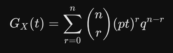
PGF for a binomial distribution
The PGF for a binomial distribution takes the form of the binomial expansion (a + b)n where a = pt and b = q:



PGF for a geometric distribution
The PGF for a geometric distribution takes the form of an infinite geometric series multiplied by pt with common ratio (r) = qt and first term (a) = 1:


PGF for a Poisson distribution
The PGF for a Poisson distribution takes a form derived by multiplying the expansion of eλt by the constant e-λ:


Mean / expectation from a PGF
E(X) = G’X(1)
Variance from a PGF
Var(X) = G’’X(1) + G’X(1) - [G’X(1)]2
Product of PGFs of independent discrete random variables
The product of multiple PGFs of independent discrete random variables is equal to the PGF of the sum of the independent variables.
For example, let X and Y be two independent discrete random variables with PGFs GX(t) and GY(t). The PGF of X + Y is equal to GX+Y(t) = GX(t) x GY(t).
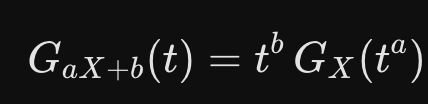
PGF of a linearly transformed discrete random variable
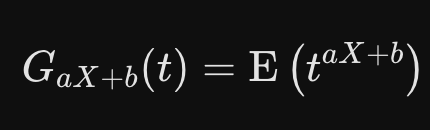
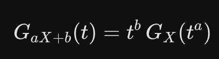
If a discrete random variable (X) has the PGF GX(t), the PGF of aX + b will be the following:
Derivation:


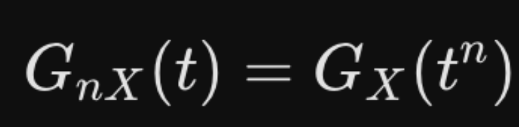
PGF of a discrete random variable multiplied by n
If a discrete random variable (X) has the PGF GX(t), the PGF of nX will be the following:
Derivation:
