Quantitative Comps Final

When the range of 95% confidence interval in Path Analysis includes 0

Indirect effect is insignificant (it may not exist)

Modification Index

An index shows how much model fit would improve, if a fixed parameter were freely estimated. Above 3.84 there can be statistically meaningful improvement.

Two approaches to modifying SEM/PA Models

Remove paths	Examine parameter estimates
	Requires careful handling (especially when removing non-significant regression paths)
	Remove non significant paths or items with low factor loadings
	Should try one by one
Add paths	Examine modification indices
	Pick up a suggestion with largest MI
	Consider if suggestion is meaningful because MI is purely based on calculation and doesn't consider theory

If RMSEA is 0 and CFI is 1

Expect just identified model (DF = 0)

Exogenous Variable

Variable is determined outside the model and determines endogenous variables

Never an outcome variable. Similar to IV.

Associated with Measurement Error

Endogenous Variable

Variable that becomes an outcome variable at least once. Similar to DV

Associated with regression residual (another type of error)

3 types of SEM and their differences and their relationship with causality and recursiveness

CFA (Confirmatory factor analysis / measurement models): No latent variables, no direct effects (regression)

Path Analysis: No latent variables, regression permitted

SEM (Structural equation modeling): Includes both latent variables and regression

They do not measure causality, rather they measure correlation and regression

They must be recursive

A non-recursive model

Has:

 Feedback loops (e.g., X → Y and Y → X simultaneously).

 Bidirectional paths between variables.

 Correlated disturbances (errors in different equations are related)

If a model is partially non-recursive, it is a bad model.

EFA acceptable data points

CFA acceptable data points

EFA: 100

CFA: Very poor 50

poor 100

fair 200

good 300

very good 500

excellent 1000

Steps for examining CFA

Collect data

Specify measurement model

Submit data to analysis

Check fit indices and parameter estimates

Modify model and re run analysis if needed

Three indicator rule for CFA

There must be at least three observed variables (items) for one factor

Each observed variable must load on only one factor

Errors of the items must be mutually uncorrelated (recall picture of errors influencing all observed variables. Errors influencing different observed variables can't be correlated

Fit indices: definition and criteria

How well the data fits the measurement model

Chi Square Test P value must be more than .05 (the null hpyothesis is that the model is a good fit for the data)

Chi Square is sensitive to sample size.

Assesses overall fit and discrepancy between the sample and fitted covariance matrices

CFI: Comparative fit index CFI must be greater than or equal to .95

Compares the fit of a target model to the fit of an independent or null model

RMSEA: Root Mean Square Error of Approximation RMSEA is less than .06

Measures the amount of misfit per degrees of freedom

SRMR: Standardized root mean square residential SRMR less than .08

If items vary in range (eg 1-5 and 1-7 scales) SRMR is better than RMSEA

Standardized parameter estimates (also known as factor loadings, show up as std.all) thresholds

Above .5 and significant (p less than .05)

Overall, to check CFA

Just check fit indexes (Chi square, CFI, RMSEA)

Then check Parameter estimates (greater than .5 and significant)

R code operators

=~

~

~~

... =~ "Load on"

Used for both CFA and SEM

~ "Regress on"

Used for SEM

~~ "Correlated with"

Used for both CFA and SEM

Multigroup CFA

Like hierarchical regression

When variables normal distributions don’t have same skewness and kurtosis

Santara Bens adjusts for this

EFA: Exploratory Factor Analysis

Creates a correlation matrix to determine what factors correlate with others. Somewhat crude

Observed items can load on to any factor.

Factors are allowed or not allowed to correlate

Errors in observed variables are uncorrelated

Factor Analysis

Goal is to find a smaller number of interpretable factors to explain the correlations among a set of variables

Smaller isn’t always better though. Don’t overreduce, but meaningless factors aren’t ideal.

Factor is a group of similar variables/items (like a construct or cluster in CA)

A summary of correlations

Dimensionality

EFA checks this

The number of latent traits, constructs, or abilities that a test is designed to assess

EFA vs CFA (Confirmatory factor analysis)

EFA: For theory/measure development (no model), weaker theories, and new measures.

Assumes a latent variable is in play and focues on identifying latent factors that explain observed correlations among variables. You extract/divide out factors from larger groups

CFA: For theory testing, stronger hypotheses/established measures.

Latent variable

A hidden or onobserved factor that is believed to be influencing something

Common factor modeling

EFA is based on

Assumes that variance in an observed variable arises from three sources

1) Common variance

2) Specific Variance

3) Measurement error.

Common variance

variance that influences multiple variables is a factor

Specific variance

variance that influences a specific factor

Key steps of EFA

Factor extraction

Identify # of factors

Rotation

Examine factor loadings

Bartlett Test

for EFA. Should be significant (assesses if there are correlations between variables/items)

KMO

For EFA: Should be .5 or higher.

assesses whether the sample size is adequate

To determine the number of factors

Recommended: Cattell Scree Test: Similar to elbow method. Find steepest line in the screeplot and select data point to the left.

Parallel analysis: Conduct a simulation and compare your data with random data. (tends to provide bigger number than other methods)

Orhotgonal Rotation

planes are 90 degrees: the planes (the factors that represent them) are unrelated and have no correlation

Varimax Rotation (recommended) is most common

Oblique Rotation

planes are not 90 degrees: this is more common, because it's used when planes (the factors that the planes represent) are related and have correlations

Promox and Oblimin is most common

Factor rotation

Factor rotation is about correlation between factors, whereas Bartlett test is about correlation between items.

Checking EFA Results: cutoff score

Sort items by factor loading and factor

Remove items that are less than .3 factor loading

Factor Loading

How much the factor accounts for the item (similar to regression coefficient)

Each variable has a factor loading for each factor

Items with a higher factor loading are more accurately measuring the factor

Orthogonal rotation range from -1 to 1

Oblique rotation: can be less than -1 or greater than 1

Typical cutoff point is an absolute value of .3

Negative factor loading indicate a negative correlation with the factor, but the magnitude is what matter (ie -.7 is a strong factor loading)

Communality

How much the factorS account for the item

When you square the factor loadings you get the communalities

In Orhotgonal rotations, they are between 0 and 1

Don’t assess if factor loadings are strong

Uniqueness

1- commonality

How much factors don't account for the item

Don’t assess if factor loadings are strong

Complexity, Low, and High

How many factors are related to an item

Range from 1 to (# of factors)

Low: Complexity is closer to 1

High: The variable is influenced across many factors (criterion overlaps with many constructs)

Complexity is closer to (# of factors)

This isn't ideal, as separate constructs will influence item scores

"You should remove items when two factor loadings are above .3

If the complexity is high, but only one factor loading is above .3, it might be acceptable to keep it

2.0 is considered a general cutoff for high complexity.

In orthogonal rotations, ranges from 0-1

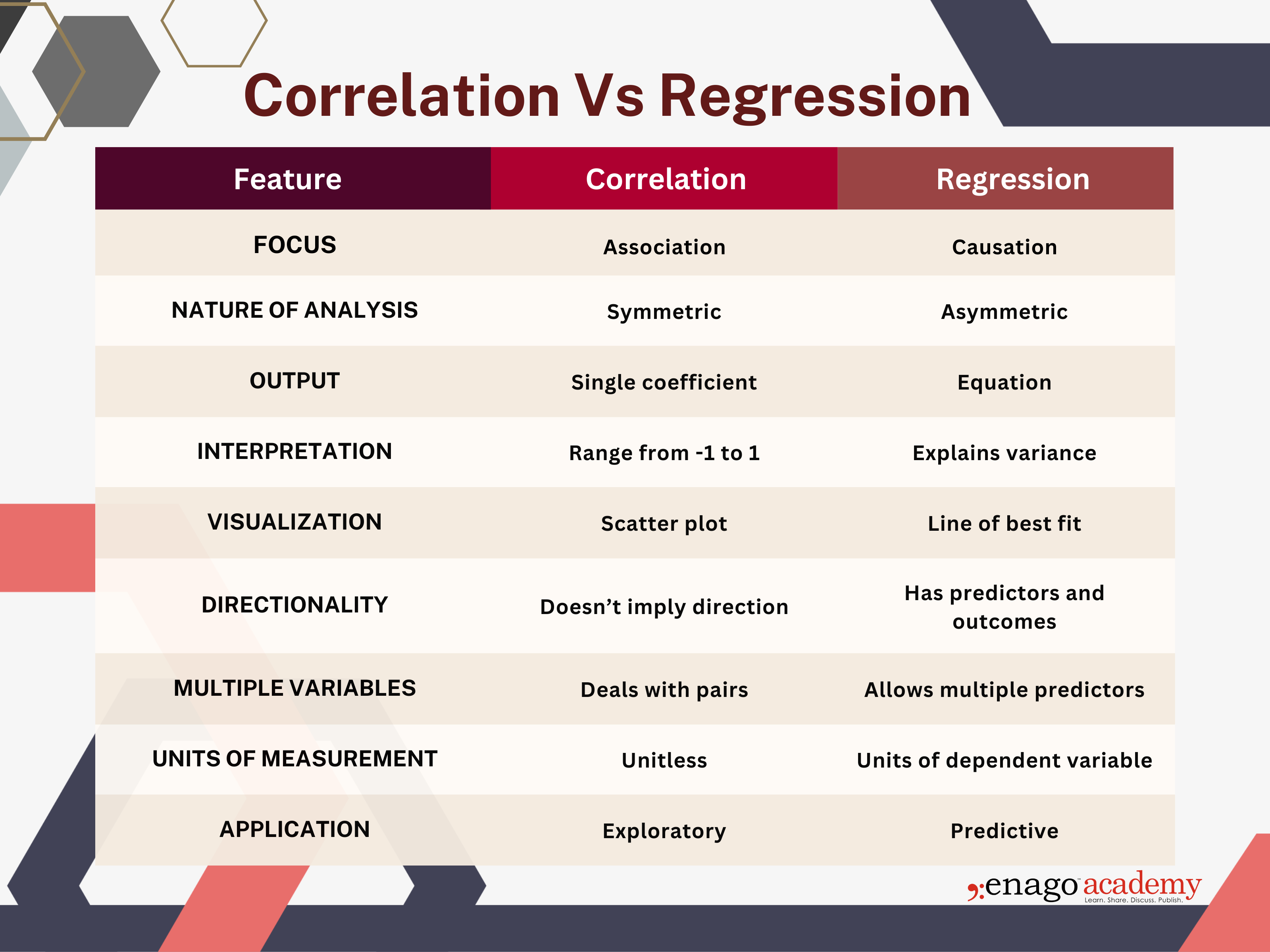
Correlation vs Regression (Focus, nature of analysis, output, interpretation, visualization, directionality, multiple variables, units of measurement, application)

Rectangle

Oval

Arrow

Double arrow

Observed variable

Latent variable

Direct effect or regression

Correlation

Direction of arrows

The origin predicts what it points to. The variance of the IV is included in the DV

CFA and cutoff point

Comfirmatory factor analysis. When your model assumes that item 1 is for factor 1, CFA assumes there is no correlation between that the item and other factors in the calculation

Estimates internal consistency

Used for examining convergent/discriminant validity

CFA is used for detecting construct bias (when construct measured isn’t the same across subgroups: detected with multigroup CFA) and differential item functioning (items work differently across subgroups)

CFA evaluates dimensionality when there are clear hypothesis
CFA Cutoff point: .5

Internal consistency unit

Cronbach’s alpha

McDonald’s Omega

Construct Bias

Occurs when a construct is measured and isn’t identical across sub groups

Can be detected by multigroup CFA

Differential Item Functioning

DIF: Items work differently across subgroups

Eg life is a party

CFA Steps

Collect data

Specify measurement model

Submit data to analysis

Check fit indices and parameter estimates

Modify model and re-run analysis if needed

CFA: Specify measurement model

Translate your hypothesis to a model

Key issues: Number of factors

Which items load on which factors

Are factors orthogonal or oblique (correlated)

Error Variance in PA and SEM

Latent variables do not have measurement error

In CFA and SEM, observed variables (indicators) always contain measurement error, which

is typically modeled as an error term (residuals)

In SEM, latent variables are often modeled with regression relationships, where

endogenous latent variables have disturbance terms (residual error) to account for

unexplained variance.

In PA: exogenous variables serve as predictors and do not have disturbance

terms since they are not predicted by other variables

Endogenous variables always have residual error (disturbance terms) since they are

predicted by other variables but are not fully explained

In CFA, latent variables themselves do not have error terms

General linear model

Generalized linear model

Generalized linear mixed model

Methods for data that's normally distributed. Assumes X and Y have a linear relationship. Examples: t-test, ANOVA, simple/multiple regression

Methods used for DV that is not normally distributed (DV is binary). Logistic regression.

Methods for nested data (hierarchical levels of grouped data). Hierarchical linear regression

Nested Data & Example

Hierarchical levels of grouped data

 Two or more than two levels

 Data cases in a lower level are included in only one higher level group (The 1st level variable is affected by the 2nd level variable)

Example:

1st level: Employee Turnover Intentions

2nd level: Economic Uncertainty

Levels

Individual, department, organization, society, etc

Mediation analysis

Tests a hypothetical causal chain where one variable X affects a second variable M and in turn that variable affects a third variable Y

Mediators & Example

How and why a relationship between two other variables

Training changes M:Self-Efficacy which in turn impacts Performance

Baron and Kenny’s 4-step indirect effect method

Step 1 Estimate the relationship between IV on DV must be significant, and effect size is not 0

Step 2 X must effect M (mediator) and the effect size must be more than 0

Step 3 M must effect Y and path must be significant and not 0

Step 4 If C' is a non significant, M is a full mediator

If C' is significant but becomes smaller, M is a partial moderator

ACME

ADE

Total Effect

ACME: Sig / ADE: Non-sig / Total Effect: Non-sig

Average Causal Mediation Effects (indirect effect, path A -> B - X to M to Y) (If insignificant, no mediator)

Average Direct Effects (path C' - X to Y)) (if significant and not 0, could have partial mediator)

Sum of Indirect & Direct Effects (not required for mediation to exist)

Indirect-only / suppression

Bootstrapping

A method to estimate the variability of a statistic by repeatedly resampling the observed data

Simulation method, more suitable for small sample sizes

Does not assume a specific distribution

P values assume normal distribution, therefore Bootstrapping is needed to assess confidence intervals by creating artificial data based on your original data set.

Sampling Distribution

The result of Bootstrapping’s artificial data creation

95% confidence interval ratio for mediation analysis after bootstrapping

If it does not include 0, it is significant

Moderation Analysis

Moderator

Name a moderator

Tests whether a variable affects the direction and or strength of the relationship between IV and DV

Moderator affects when a relationship occurs

Workload - perceived social support - burnout

Moderated mediation (more common)

When there is a moderator that affects a mediator's relationship with Y

Starting point is the moderator and the IV

Example: Ability influences performance and is mediated by job knowledge but it is stronger when supervisor support is high

Mediated moderation

Take the L

Centering

Center the IV and Moderator W before estimating the model

Transfer a variable so that its mean becomes 0 by subtracting the mean

Subtracts the mean of a variable from each value in that variable

Reduces multicollinearity and make interpretation easier

Makes main effects interpretable

Multiple Regression vs Logistic Regression

MR: DV is a quantity and ranges to infinity (continuous or interval data) and has a linear relationship with IV

LR: DV is 0 or 1, and calculates probability. Uses logarithmic transformation to Y to linearize relationship between IV and DV

Why not use MR when you have binary DVs?

If you use MR for dichotomous DV, it violates heterogeneity of variance/homoscedasticity (MR assumes variance of errors remains constant across all values of X, but binary DV violates this assumption (close .5 probability, error variance is large, close to 0 or 1, EV is low.) A one unit increase in X does not lead to a fixed increase in Y.

MR can produce DV estimates greater than 1

Linear models can’t express slope of probability varying depending on IV

Turnover analysis Pros/Cons of

Group Comparison (T-test)

Correlation

Regression

T-test: Test one variable at a time, hard to discern importance

Correlation: Which variables are related to turnover? Outcome is binary, so correlation is unclear

Regression: Can predictors explain turnover? MR assumes continuous variables, but outcome is binary

Odds

The likelihood of an event occurring compared to the likelihood of it not occuring

Odds ratio & Interpretation

Comparing the odds between two groups, with the reference/baseline group as the denominator.

OR>1 Event is more likely in the numerator group than the reference group

OR=1 Event is equally likely in both groups

OR<1 Event is less likely in the numerator group than the reference group

OR with continuous predictor

Interpret as, “what happens when X increases by 1 unit.”

OR = Odds at X+1 / Odds at X

Marginal Standardization Approach (MSA)

In Logistic Regression, probability changes are not constant. They depend on the starting value of X.

Two methods:

1: Specify the starting point (a 1 unit increase in X changes Y (probability) to _%

2: Use the average effect (average marginal effect (AME)) (On average, a 1 unit increase in X changes probability by _ percentage points.

Adjusted R Squared

Shouldn’t be interpreted, but can be compared. Nagelkerke’s and McFadden are common

Logistic Regression Assumptions & Pairwise Deletion

No outliers, no multicollinearity, DV is binary, Appropriate sample size, no perfect separation, independence of observations, linearity of log odds relationship

Pairwise shouldn’t be used in LR: Violates Maximum likelihood estimation assumptions, inconsistent sample size, unreliable standard errors. Use Listwise deletion or multiple imputation.

LRT: Likelihood Ratio Test

Equivalent to F test in linear regression

Compares the full model with a null (intercept-only) model

Evaluates overall model significance

Reported as Chi Square statistic

Can assess contribution of individual/significance of predictors

Wald Test

Focus on Statistical significance of predictors

Beta Coefficients indicate direction and can be compared across predictors (OR > 1 increases likelihood, OR < 0 decreases likelihood of outcome

CI doesn’t include 1: statistically significant

Hosmer-Lemeshow Test

Sensitive to large sample size

P is insignificant (> .05): Model is acceptable

Compares predicted probabilities with observed outcomes.

Callibration plot

Above and below the mean indicates…

Evaluates how well predicted probabilities match observed outcome frequencies. Predicted is X, Observed is Y

Above the line: Underestimates

Below the line: Overestimates

ROC Curve and AUC (Area Under the Curve)

Evaluates predictive performance

AUC ranges 0-1. 1 is perfect prediction.

.7-.8 is acceptable

.5-.7 is poor.

less than .5 is worse than random prediction

Accuracy

How often is the model correct overall?

Proportion of correctly classified cases

Sensitivity (True positive rate)

How well does the model detect the event?

Specificity (True negative rate)

How well does the model detect non-events.

Sensitivity and specificity

Are inversely related. The cutoff point leads to a trade-off

Determining cutoff point

Can be determined using Youden’s Index

Sensitivity+Specificity-1: optimizes Maximizes balance between

Or ROC Curve (AUC):

Point closest to the top left corner

Pulse Survey & Benefits

5-15 items

Weekly/quarterly

2-5 minutes

Specific focus

Benefits: Low burden/high response rate, Real time insights/detect issues early, quicker improvements, Monitor change

Survey Limitations

Survey fatigue

Limited opportunities

Poor design (not actionable, poorly formatted for analysis)

Good surveys are designed

Backward from action

If your survey doesn’t lead to action, it has little value.

With validity, reliability, and practicality in mind

To average and compare across time/depts/benchmarks/tenure.

Surveys can include

Interviews, focus groups, and open-ended feedback.

Engagement surveys, pulse surveys, exit surveys/interviews, onboarding surveys

Methods vary.

Surveys communicate

Organizational values and priorities

Shape norms, culture, and expectations

Item Format: 4 vs 5 items

-Response flexibility (allows for uncertainty or neutrality)

-Reduced response bias

-Reduce respondent’s stress

Costs and benefits of Open and Closed Items

Open:

Cost: Difficult to analyze, time consuming

Benefit: rich details, can capture ideas not on researcher’s radar

Closed:
Cons: Limit respondent’s thinking

Benefit: Faster to analyze

Acquiescence

People who select agree to all items

If questions have

Multiple reasons

Everything is important

There may be unexpected responses

Multiple answers

Ranking

Open-ended

What are you trying to measure

Attitudes/perceptions

Behaviors

Reasons/background

Priorities

Applicable factors

Likert

Frequency

Open-ended

Rank-order

Multiple answers

Should you include both positively and negatively worded items in a survey

yes: Avoids acquiescence, careless responding

Bad: Can create reverse items

Leading vs Loaded Questions

Leading: Guides respondents toward a specific answer

Loaded: Contains an unverified assumption

Ambiguous

Too long

Pedantic

Multiple negative

Double barreled

Ambuous pronoun references

Misplace modifiers

Adjective forms rather than noun forms

Four Types of Data & Definitions

N: Nominal: Categorical identity - Mutually exclusive data. Example: Freshmen, Sophomore, Junior, Senior.

O: Ordinal: Order - Interval isn't consistent. Always starts with 1. Example: Top 3 candidates for a job

I: Interval: Assesses a degree of quantity in addition to identity and order. Zero doesn't mean nothing. Example: Temperature

R: Ratio: Assesses quantity, identity, order, and Zero means nothing. Example: Distance, Mass.

T Tests

Compare two means from two seperate populations. Outcome variable is ratio or interval. Results in a T score (like effect size) and p value (significant indicates a meaningful difference between groups)

Chi Squared Tests

Compare two categories, or two nominal forms of data (if three groups, use ANOVA). Results in a p value and X squared effect size indicator

Independent Samples T-test

Between subjects test (there are multiple groups, or different populations. 1 control doesn't receive the IV, and you compare their results to another group that does)

Paired Samples T-Test

Within subjects test (you're assessing something within one population, usually measuring something, applying the IV, then measuring the same thing again)

How to check for normality (and what is distribution)

Shapiro Wilk Test (If p > .05 assume normal distribution) or QQ plot (straight line equals normal distribution)

Distribution: the overall shape of the data, shown via graph. Think entire mountain range, peaks & valleys

How to check for variance (and what is variance)

Levene’s test: Assesses if two populations have equal variances. if p > .05 assume equal. If p < .05 assume different variances. If unequal variances, use Welch's test

Variance: A single numerical value that quantifies the dispersion of a distribution. A low variance indicates that data points cluster closely around the mean, while a high variance means the data points are scattered far away from the mean. Think: 1 number indicates the degree of flatness