Ch 5 - CPU scheduling - Part 1 - Lecture Vid

Basic Concepts

So first, any process running on the CPU always has either a CPU burst or an I/O burst. Some of the code segments, some of the instructions, require a lot of CPU computation. On the other hand, some other instructions may just be waiting for the I/O devices to finish. Note that the I/O devices are way slower than the CPU most of the time. So when the program or process is waiting for the I/O system or I/O devices to finish their work, then really these processes are not doing anything in terms of CPU usage. Why? Because these devices are slower than the CPU. That means the processes waiting for the I/O device, if they continue running on the CPU, are not really using the CPU and are wasting a lot of CPU cycles. So we need an efficient way to switch the processes so that we can always keep the CPU busy doing computation tasks, while the processes waiting for the I/O devices may wait in the I/O device queues so that they don't take CPU cycles. So that's the goal of the scheduling.

Histogram of CPU-burst Times

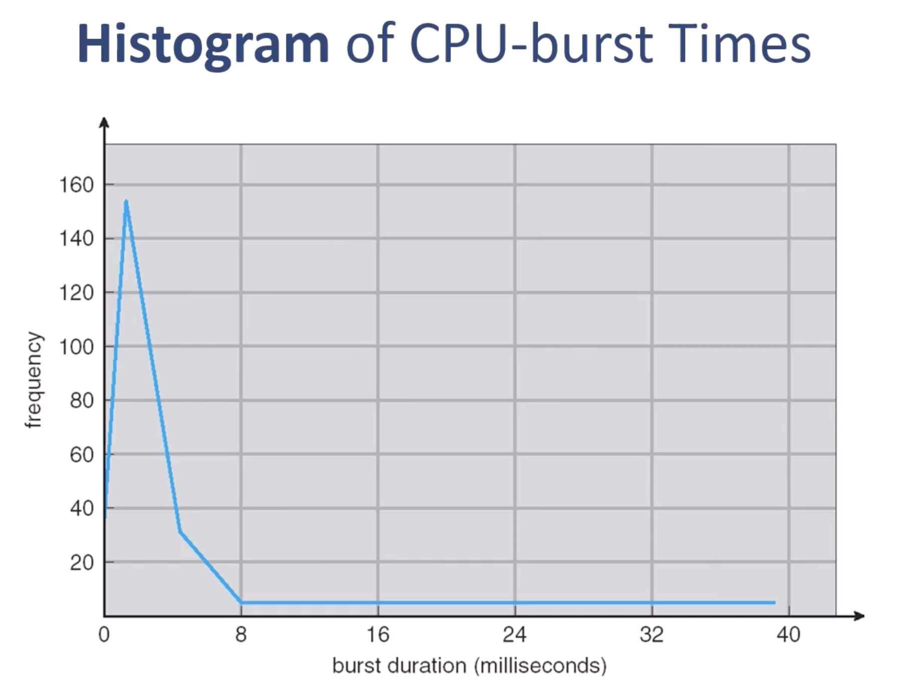
When we draw a histogram of how much frequency, okay, how many times a particular CPU burst happens throughout a process's life cycle, and also considering all the processes and all the CPU bursts in an operating system, then on average what we see is a lot of short CPU bursts happening, while longer CPU bursts happen rather rarely. So you can see a huge spike here, right? And that means that processes often have, most of the time, the CPU burst time is rather short. It's about less than 4 milliseconds, okay, less than 4 milliseconds. And the longer CPU burst times, they don't happen that much. So regarding the CPU...

CPU Scheduler

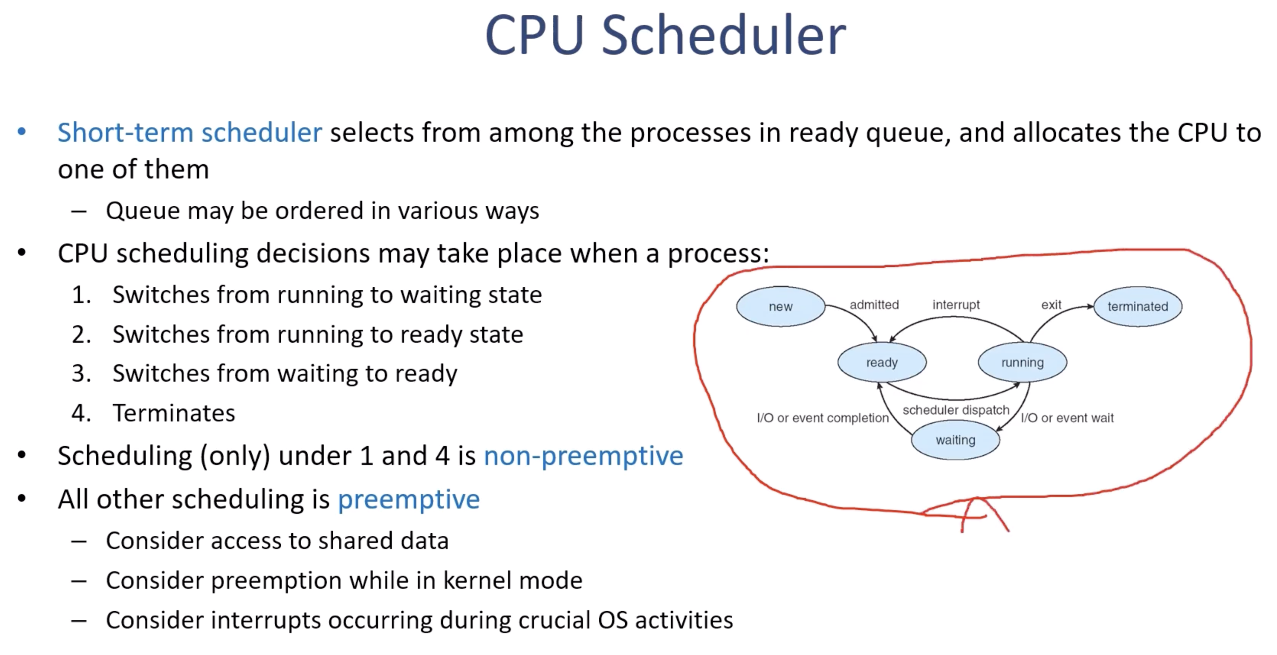
So in this textbook, we learn a process's life cycle as five states. So they first create it and then admit it into the ready queue, and then start running the CPU if the scheduler dispatches the process into the CPU. And sometimes the process is interrupted by another process for various reasons, and in that case, then the process has to be added back to the ready queue. Or if the process requests I/O, then they have to go into the waiting queue of the I/O device, and waiting becomes a waiting state. When they are done with the I/O device operations, then they are admitted back to the ready queue so that they can take the next CPU cycle. And then when they are all done with all the computational tasks, then the process can be terminated. So really, in this chapter, what we focus on is the short-term scheduler that selects the process among the processes in the ready queue, which is this guy, okay, which is this guy, and then we allocate the CPU to one of them. And the CPU scheduling decisions may take place when a process does one of these four things. So number one is switching from the running to the waiting state. So running to waiting state, that's one thing. Or switching from the running to the ready state, so when the interrupt happens. And the third is switching from waiting to ready. So waiting to ready, then the process who was waiting for the I/O device to finish its job gets into the CPU's ready queue. Or the process terminates. Okay, so if any of these four things happen, then the CPU scheduler takes the appropriate action to switch the processor around. And scheduling under condition one and condition four, they are the nonpreemptive actions. So when a process switches from the running state to the waiting state, that is voluntary, because the process has requested some I/O operation. And that means, just looking at the instruction type, if the instruction is requesting I/O, that means we can easily say that the process does not need the CPU right away, and it can be safely taken out of the CPU and get into the waiting queue for the I/O devices. So that doesn't require preemptive control. Another condition is, this is pretty obvious, when the process finishes all the instructions, then the process is done and it's terminated. So that's another condition that the process will voluntarily release the CPU. So those two are the nonpreemptive scheduling decisions. On the other hand, the other two situations, the scheduling should be preemptive. So we need to consider access to the shared data, we need to consider preemption while in kernel mode, or consider interrupts occurring during crucial operating system activities. So when this context switch...

Dispatcher

When this context switch happens, then a dispatcher module, a hardware device called a dispatcher module, gives control of the CPU to the process selected by the short-term scheduler. And this involves the actual context switch, as well as switching to the user mode and jumping to the proper location in the user program to restart the program where it should start. So this dispatcher module hardware is important in this context switching to be implemented. And of course, this doesn't come free. So when this dispatcher module is involved in this context switch, that requires some delay that introduces some delay in processing, and that is called dispatch latency. And we will revisit this time, okay, to take to do the context switch later again when we discuss the real-time schedulers.

Scheduling Criteria

(goal is to make CPU as busy as possible)

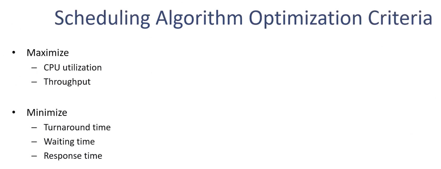
Now before we look into the actual algorithm choices, let's see what are the criteria that we can use to compare the different choices of algorithms. So we will basically use five different criteria in the textbook. The number one is CPU utilization. This is in percentage: how much time the CPU is busy. So if it says 100%, that means CPU utilization is 100%, which means the CPU is always busy. Okay, and if it is 80%, that means about 80% of the time the CPU is busy, and it has 20% extra room to run any other processes or computation tasks. Task throughput is another measure that measures the number of processes that complete their execution per time unit. So, for example, within one minute, how many processes were able to finish using that particular scheduling algorithm? If one scheduling algorithm A was able to finish 10 processes within that one minute of time, then that is probably better than another scheduling algorithm that was able to finish only five processes within the same amount of time. So that is another criterion that we can use to compare the different schedulers. By the way, CPU utilization, how can we tell that one scheduling algorithm is better than the other scheduling algorithm using CPU utilization? Because our goal of the scheduling algorithm is to make the CPU as busy as possible. So if scheduling algorithm A most of the time has 90% CPU utilization on average, and scheduling algorithm B just has about 75% CPU utilization on average, then we can say that scheduling algorithm A is better. The other scheduling criteria are turnaround time, waiting time, and response time. Let me go over each one of these one by one. So turnaround time means the amount of time to execute a particular process. So that is the summation of the time period spent while getting into the memory, waiting in the ready queue, actually executing on the CPU, and doing all the I/O. It includes the entire amount of time to execute the program. That is the turnaround time. So that means the time that you click on that program icon and it starts running, and the time that you press X or the program finishes. So the entire duration of the process's runtime, that is the turnaround time. Waiting time, on the other hand, is the amount of time a process has been waiting in that ready queue. So that means the waiting time is actually included inside the turnaround time. And among the entire time of execution, the entire turnaround time, some of the time frames, some of the time within that time frame, the process is not doing anything and is just waiting in the ready queue. Okay, waiting in the queue for the next CPU, waiting for the next CPU cycle, and waiting time measures that amount of time. So how much time is the process waiting around in the ready queue and not doing the computational task? Okay, so that's the waiting time. Response time is yet another measure that is the amount of time it takes from when a request was submitted until the first response is produced. And that doesn't necessarily mean that the processor has to create an output, a visual output. So the best example of response time is the time duration between the point that you double-click on your icon until you see the window pop up on your desktop. So that could be a response time. But not necessarily, as the definition says, it is not necessarily the output; it's the first response that is produced. So anyway, that is the response time, and the waiting time and the turnaround time. Those are the other three scheduling criteria that we can use to compare different scheduling algorithms. So for each different scheduling algorithm choice, say algorithm A, B, C, D, you can measure these five criteria and compare each other and see which one is better than the other. I already explained the CPU utilization and throughput examples. How about turnaround time, waiting time, and response time? Yes, if the turnaround time, waiting time, or response time is smaller, then you can say that that algorithm is better than the other. So in other words, I have a good reason why I put the space in between these two and these three. The top two are something where higher is better, okay, the larger the better.

Scheduling Algorithm Optimization Criteria

On the other hand, those three, the bottom three, they are smaller the better, okay? So all these five criteria are what you can use to compare the scheduling algorithms, but the top two are higher the better, and the bottom three are smaller the better. All right, so our goal is to maximize the CPU utilization and throughput while minimizing the turnaround time, waiting time, and response time.

First-Come, First-Served (FCFS Scheduling)

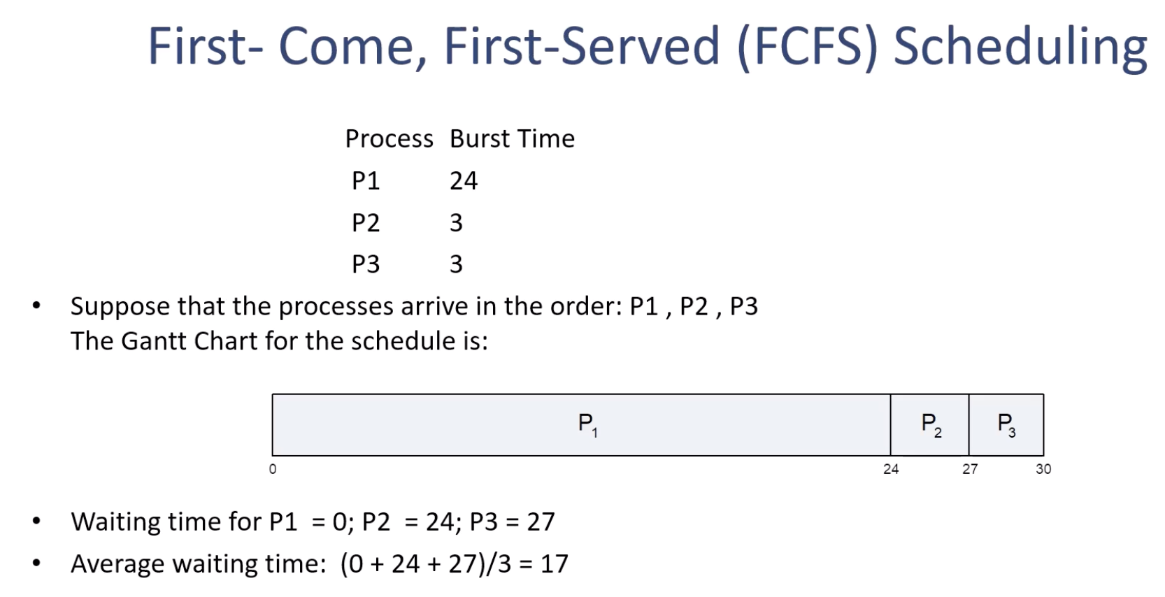
Now armed with this scheduling criteria, we can now discuss some of the representative scheduling algorithms that we can use in operating systems. The first algorithm is very easy. It's a First-Come, First-Served algorithm. Note that it's not First-In, First-Out, okay? So the term is not First-In, First-Out. Although the concept is the same, the correct terminology we use for the scheduling algorithm is First-Come, First-Served, or FCFS scheduling algorithm. Like the name says, it means that we process the processes as they come in. So let's say we have three processes, Process 1, 2, and 3. They come in in exactly this order, with virtually no delay between them, and then Process 1 burst time is 24, Process 2 is 3, and Process 3 is 3. Okay, let's assume that their burst times are like this. For the burst time, we use the measure of milliseconds in this chapter, so they are in milliseconds. Now suppose that they arrive in this order, and then we can draw the Gantt chart, how these processes are admitted and run on the CPU. So Process 1 runs first, Process 2 next, Process 3 next, okay? Pretty easy. And then you can draw the timeline like 0, 24, 27, and 30. Okay, now then what is the waiting time for Process 1? Process 1 gets into the ready queue and starts running right away, so that's zero. Process 2 waited for Process 1 to finish, so that means 24. Process 3 similarly waited for 27 milliseconds. That means the average waiting time of these three processes is (0 + 24 + 27) divided by 3, which is 17. Okay, how about Process 2 and Process 3 arrive before Process 1?

FCFS (cont.)

Like this, what is the waiting time for Process 2, Process 3, and Process 1, and what is the average waiting time? You may, for the entire chapter of this topic, the scheduler chapter, when questions are given like this, I strongly recommend you to pause the video and try to calculate on your own, and then continue or resume the video to see what the answer is. Okay, so Process 1 waited for 6 milliseconds, right? And Process 2 waited for nothing, and Process 3 waited for 3 milliseconds. That means they waited for this amount, and divide by 3, that means 3 milliseconds on average. Okay, 3 milliseconds on average. So that means that is much better than the previous case. In other words, depending on the order of process arrival, our average waiting time, in other words, the First-Come, First-Served scheduling algorithm's performance varies a lot, okay? Varies a lot. This is called the convoy effect. When the short process is behind the long process, then the average waiting time will skyrocket, and your scheduler's performance will degrade, as you saw in the previous slide. So that means the First-Come, First-Served scheduler is not ideal for a system that requires really robust and reliable performance, reliable and consistent performance. So we need a better idea.

Shortest-Job-First (SJF) Scheduling

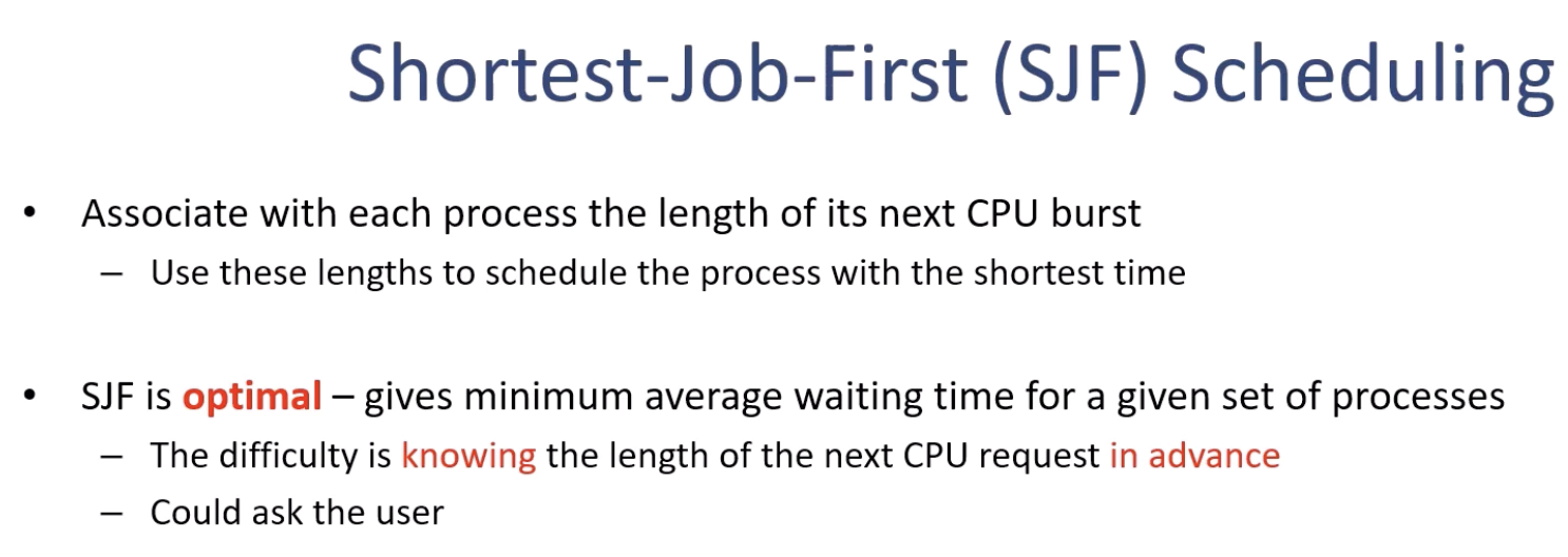
The second scheduling algorithm that we will learn is what's called the Shortest Job First scheduling. We associate with each process the length of its next CPU burst. We use these lengths to schedule the process with the shortest time first. So the scheduler selects the process with the shortest CPU burst. Because the convoy effect is problematic when a process with a short CPU burst comes after a process with a long CPU burst, why not give the CPU burst time an inversely proportional priority? So that means the shorter CPU time means higher priority, and we give the priority to those processes. Interestingly, the Shortest Job First algorithm is optimal. You can't do better than this, so it gives the minimum average waiting time for a given set of processes. So that is pretty good. Okay, so does that mean we solve the problem? The answer is actually no, and that's because it's very difficult, almost impossible, to know the future in advance, unless you are an oracle. So that is one big problem. It's just in theory, on paper, that Shortest Job First is optimal, but in practice, that's not possible. Maybe you could ask the user in advance how long your process would take, say, for example, but that is not feasible in all cases either, because even users may not know the exact amount of CPU burst time before they actually run it. And even the same process may take different amounts of time depending on the condition of the hardware and other processes running at that given time. So really, it is impossible to know the future. So once again, Shortest Job First is optimal, but it's only theoretically optimal, and in practice, it's impossible to predict the future.

Example of SJF

Anyway, let's see how good Shortest Job First is. Because it's good to know, it's good to practice at least and learn what it is, because with this we know exactly what the best we can do is, given any situation when we are designing any new scheduling algorithm, right? So we know the best, the upper bound of what we can do. So let's see what is the average waiting time for the scenario given in the slide using the Shortest Job First algorithm. So we have four processes, 6, 8, 7, 3 burst times, and then we can draw the Gantt chart like this. What is the average waiting time? For Process 1, it took 3 milliseconds; Process 2, 16 milliseconds; Process 3, 9 milliseconds; and Process 4, 0 milliseconds. So they waited for this amount of time. What you can do is just add this up and then divide by four, which is 7. So what is the average waiting time using First-In, First-Out, or more precisely, FCFS, First-Come, First-Served scheduling algorithm, in this case? Can you do it? So we can write P1, P2, P3, P4 like this, and the tick values are 0, 6, 14, 21, and the last one is 24. So they waited for 0, 6, 14, and 21. That means you can add up 6, 14, and 21, divide by 4, which is 41 divided by 4, so that's about 10.25, which is way better. Okay, so you can see that is way better. So then Shortest Job First is way better than First-Come, First-Served.

Determining Length of Next CPU Burst

Okay, now let's determine the length of the next CPU burst. Why do we want to do this? Well, we don't know the future. There's no way we can know the exact future in the real sense, but what we can do is maybe estimate the possible length of the next burst. That's based on historical information. So we can learn from history and then try to predict what's going to happen in the near future. So an algorithm that we can use to predict that future is what's called exponential averaging. And the calculation looks like this. Initially, we make an assumption, and then we come up with some parameter. We predefine a parameter that determines how much weight we are going to give to the historical information versus the up-to-date information, right? And then based on that, we make the next estimate as a ratio, okay, a weighted sum of history and the up-to-date information of this CPU burst. Commonly, this alpha value is set to half. That means we give the same weight to the history and up-to-date information. And a preemptive version of using this exponential averaging estimate of the CPU burst is called Shortest Remaining Time First, or SRTF.

Prediction of the Length of the Next CPU Burst

So here's an example of how this prediction works, how exponential averaging works. Our initial guess, let's say, is 10 milliseconds. And then we observed the actual CPU burst of the process, and let's say it was 6. Then by taking half and half, we basically take the average of it, and it becomes 8. And then let's say our next real observation was 4. By taking half and half, we get the average of 6. Next time, we actually got the right prediction, so the real one is also 6. That means taking the average of the two, we stay with 6. Okay, and then like this, we can keep updating the value. And when we make a big mistake, then gradually, gradually, we approach the new observation. Okay, so that's why we end up with this smooth curve that makes a reasonably good prediction of the next CPU burst.

Examples of Exponential Averaging

And let's see a little bit more detail on what these alpha values mean. So the alpha, when it is zero, that means the formula, the original formula, by the way, that's here, okay, the original formula becomes what? When alpha is zero, then the first term goes away, so then we only have the second term, okay, the second term. Starting with t₀, t₁ is what? t₁ is (1 - 0)t₀, okay, and t₂ is (1 - 0)t₁. In other words, they don't change, okay? They don't change at all. In other words, when alpha is zero, then we do not care what actually happens in the real system, and then we just keep the original estimate, we just keep the original guess forever. If the alpha is one, that's another extreme. By the way, the alpha should be between zero and one, inclusive. And when alpha is one, that's the opposite case. So in that case, the history term goes away, and then we only use the first term. So t₂ is alpha t₁, and t₃, but alpha is one, so that's basically t₁. Alpha 3 is t₂, and so on. In other words, tₙ₊₁ is basically the same as tₙ, and that means we only care about the actual most recent CPU burst as our estimate, and we completely ignore the old history. So that's the other extreme case of this exponential averaging when alpha is one. Now we can expand the formula. So we start with the original formula, this original update formula, like this, and then we can gradually expand this. So tₙ is what? tₙ is alpha tₙ₋₁ + (1 - alpha)tₙ₋₁, and then we can further expand this guy, okay, further expand this guy. So after simplifying this, the second term, the second line, then we get this, and then we can now further expand this by rewriting that tₙ₋₁ is alpha tₙ₋₂ + (1 - alpha)tₙ₋₂, and so on and so on. We can keep going. Then we can come up with a general form of all these terms here. So the first term is alphaⁿ. The second term is (1 - alpha)alphaⁿ⁻¹, and then in an arbitrary term, the j-th term, that means (1 - alpha)alphaʲ, okay, and for tₙ₋ⱼ. Note that this one can be considered as tₙ₋₀, this one tₙ₋₁, and that's n - 0 and n - j. Now we can see the last term, the initial t₀, is multiplied by (1 - alpha)alphaⁿ⁺¹. Why? So you can see that if we start with one, right, we start with one, and this is actually (1 - alpha⁰), okay, and (1 - alpha¹) and (1 - alphaʲ). So that means the last one, when n - 0 becomes zero, this value is this guy, right? So this guy should become n + 1, okay, n + 1. So for that, what can we tell? What can we say about this? What we see here is the alpha here is always the largest value, and then we keep multiplying some value that is between 0 and 1 again and again to this coefficient alpha until we get (1 - alpha)alphaⁿ⁺¹. Obviously, this number is way smaller than this, and the number will keep becoming smaller and smaller because we are multiplying a number that is between zero and one, right? So that means we are giving smaller and smaller weight on the history as the history becomes older, and the very initial guess, the initial guess we give the smallest weight when calculating the estimate for the new value, the estimate for the new CPU burst. So since both alpha and 1 - alpha are less than or equal to one, each successive term has less weight than its predecessor. In other words, we are giving less and less weight to the history, or older history, and give more weight to the more recent history, which makes perfect sense. So that's how the exponential averaging works.

Example of SRTF

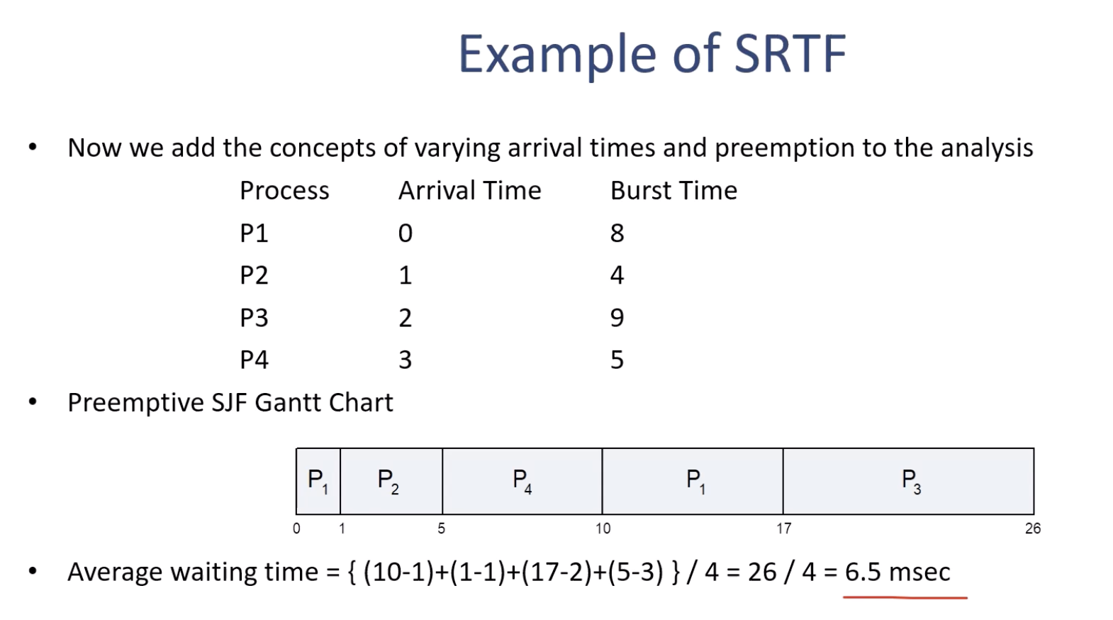
The next algorithm we will discuss is the Shortest Remaining Time First algorithm. This is based on our burst time prediction, okay? So, burst time prediction. So now we have a way to predict the burst time. We can attach this predicted burst time here, and then we can also consider the arrival time of these processes. So the processes do not have to arrive, we do not have to assume the processes all arrive at the same time, at time zero. Rather, they may arrive at different times, and then we can consider how much time is left, how much burst time is left for these processes. And based on that, we can decide which process at that given time, okay, at that given time, which process has the smallest remaining time, okay? So, shortest remaining time left, and then we can choose that one first. So that eventually we are mimicking the behavior of the Shortest Job First algorithm. So at the beginning, we have process one arrive at time zero, and its burst time is eight. So since no process is there, it's obvious we can start with process one. After one millisecond, process two arrived. At that time, process one's remaining burst time is seven because it has executed for one millisecond. And now that we are comparing process one and two, which are seven and four, which one is smaller? Yes, it's process two. So we are running process two at this time. So process two can start running. After another millisecond, at two milliseconds, okay, at two milliseconds here, at that time process three arrived. At that time, how much burst time is left for all the processes? Process one still has seven milliseconds left. Process two now has three milliseconds left, and process three just arrived and needs nine milliseconds. So that means process two can continue running. And after yet another one millisecond, then process four arrived. And at that time, process one still has seven milliseconds, process two now has two milliseconds left, and then process three has nine milliseconds, and process four, which just arrived, needs five milliseconds to finish, right? So that's where it is, and that means process two can continue running and should finish in two additional milliseconds. Okay, so when process two finishes, that is the fifth millisecond here. Okay, that is the fifth millisecond, and then finally process two is gone. Now we can decide among process one, three, and four to decide which one should run next. And because it's the Shortest Remaining Time First algorithm, among process one, three, and four, process four should run next. So it runs for five milliseconds, so that's ten milliseconds here, and then process one, that's seven milliseconds, and then process three, which is nine milliseconds. So what's the average waiting time? Average waiting time is here, you need to be a little bit careful because not all processes arrive at the same time. So process one arrived at time zero and then executed for one millisecond, and until it starts running again, it waited for this amount of time, okay, which is nine milliseconds. So process one waited for nine milliseconds. How about process two? Process two waited for nothing, so that's zero milliseconds. Process three waited for how long? It arrived at two milliseconds and then started running at seventeen milliseconds. So that means process three waited for fifteen milliseconds. And process four arrived at the third millisecond and started running at fifth millisecond, so that means it waited for two milliseconds. Okay, so if we add these numbers up, that is twenty-six milliseconds, and divide by four, we get 6.5 milliseconds. So that is the average waiting time of these four processes using the Shortest Remaining Time First algorithm. Okay, all right.

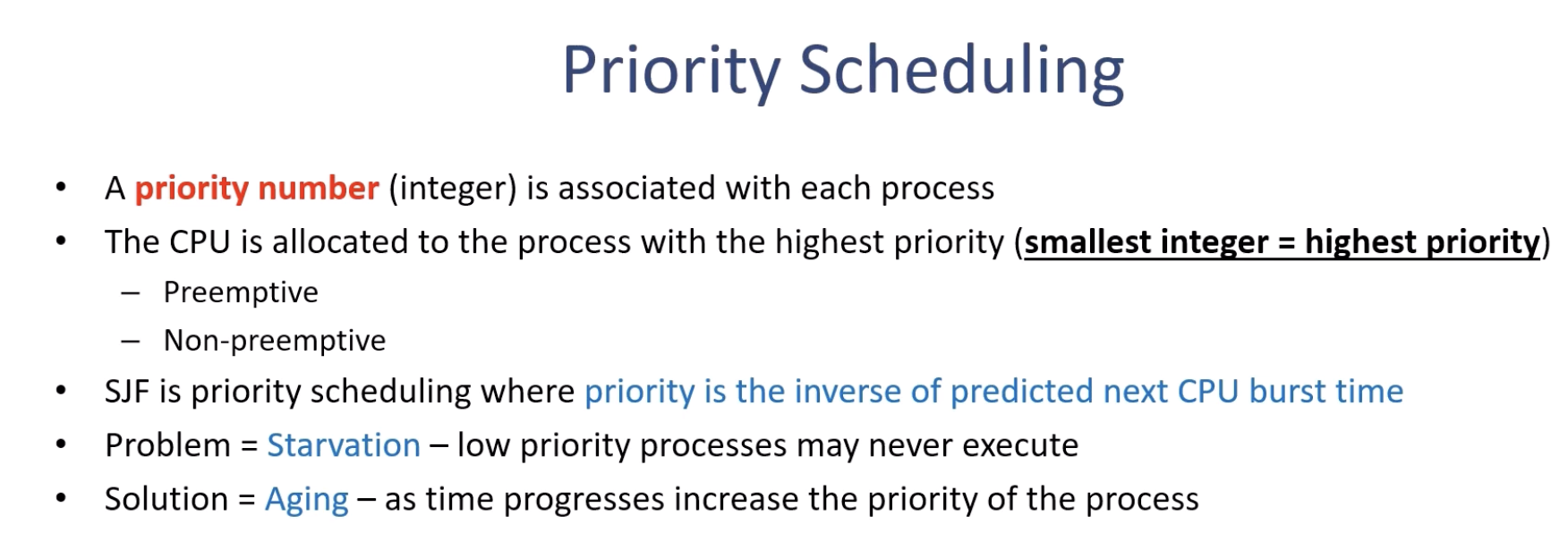
priority scheduling