Ecology Unit 1

The 3 D’s

Distribution, dispersion, and density

Ecology

the scientific study of the relationships between organisms and their environment

Population

a group of (interbreeding) individuals found in the same space or area at the same time (must include area and time in definition)

Demography

the study of the age structure and growth rate of populations

Density

the number of individuals in relation to the space or volume in which they occur

Distribution

the geographic and ecological range of a population

Dispersion

the spacing of individuals with respect to one another

Mark-recapture methods

• Individuals (numbering M) are captured, marked, and released.

• We assume that they mix freely and completely with the rest of the population.

• Then we capture some individuals again

• Count the total number of individuals caught (n) and the number of those that were marked previously (x).

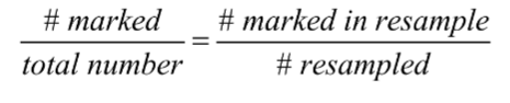
What problems exist with this mark-recapture method?

It made certain (poor) assumptions about:

-- distribution

-- dispersion

-- better with more marked individuals and larger re-sample

Population pyramids

\
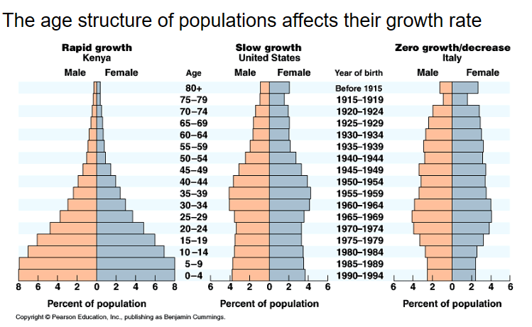
demographic transition

as countries develop their economies, they shift from something like Kenya to something like the US

Case studies: Sir Ronald Ross

Sir Ronald Ross used linked equations to study malaria

On August 20th, 1897, Sir Ronald Ross, while working as a military physician in India, demonstrated the malarial oocysts in the gut tissue of female Anopheles mosquito, thus proving the fact that Anopheline mosquitoes were the vectors for malaria.

\
**Ross also tried to predict the spread of malaria** in human populations. He created two linked equations, one each for infected humans (H) and for infected mosquitoes (M).

dH/dt = # new human infections - # recoveries or deaths

dM/dt = # new mosquito infections - # mosquito deaths

(Note the dN/dt = births – deaths form!)

\

b= per-capita birth rate

the probability of an individual having offspring during some time period

bN

Population birth rate

We can just multiple each of these per-capita rates by the populations size (N) to get a rate for whole populations

d = per-capita death rate

the probability of an individual dying

dN

Population death rate

We can just multiple each of these per-capita rates by the populations size (N) to get a rate for whole populations

population growth rate (dN/dt)

dN/dt = population births – population deaths \n

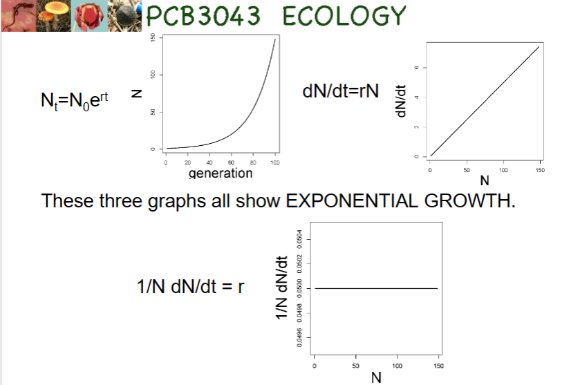
dN/dt = bN – dN \n (note confusing use of “d” for two different things here!)

Immigration

individuals that join the population

Emigration

individuals that leave the population

exponential growth

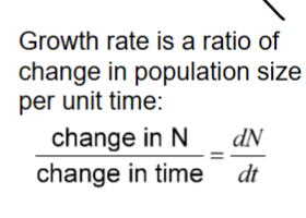
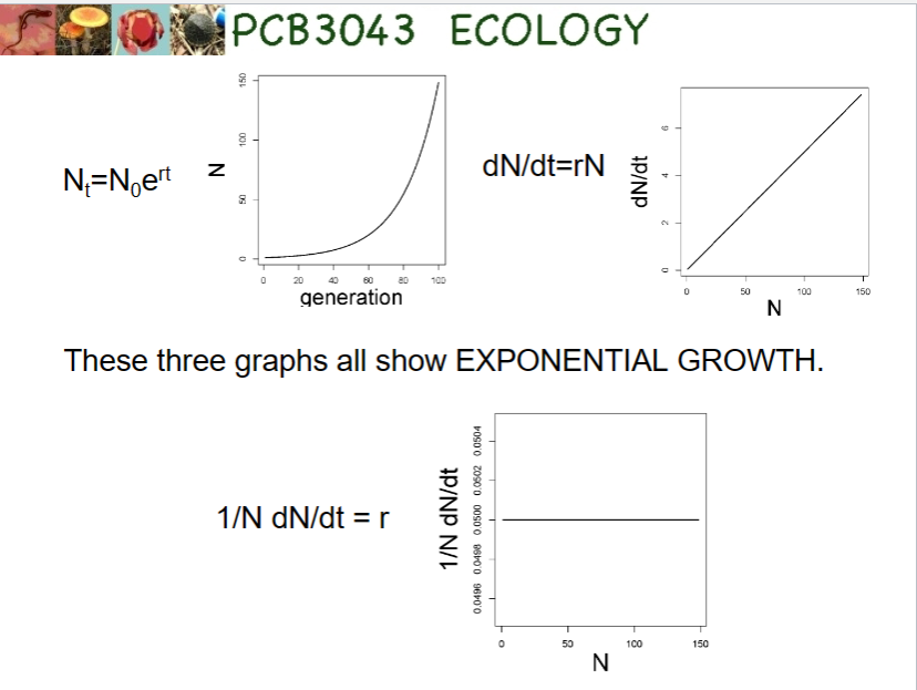
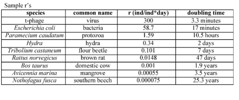
“little r”

r = births – deaths + immigration – emigration

per-capita growth rate

the intrinsic rate of increase

we get exponential growth with continuous growth if r remains constant and positive

What does r equal when the population is increasing?

positive

What does r equal when the population is decreasing?

negative

What does r equal when the population is stable?

0

closed population

If there is no movement of individuals between different populations, (no immigration or emigration) then the numbers of individuals are determined by local processes (that is, just births and deaths)

open population

alternatively, if there is significant movement of individuals between populations, then the population is considered to be open

Expected little r for different species

Little r is instantaneous and can be used to compare growth rates

THE MAJOR PRINCIPLES OF POPULATION ECOLOGY

(1) Populations have the potential to grow rapidly.

(2) They usually don’t. Populations must be regulated such that rapid growth is a transient, but common phenomenon

John Graunt and population demography

John Graunt’s study of the growth of London, used to predict the population of the world

\
His worked showed the two laws of population growth

Discrete Growth

everyone overwinters as an adult, finds mates in the spring, has babies and dies. At any point in the year, all individuals are about the same age.

Nt+1 = Nt x R0

Note that since it is multiplicative, if R0 = 1, the population is stable

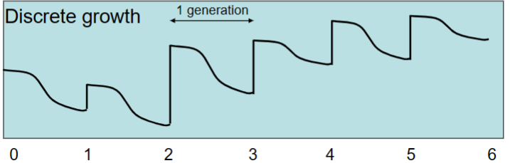
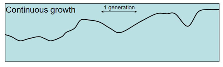
Continuous growth

reproduction is not tied to seasons and can go on at any time. Individuals have might live just as long as before, but they can mate, make babies, and die all year round

R0

R0 (“R sub O”) is another growth rate, if R sub 0 is constant, exponential growth.

If R sub 0 is 1, population is stable

Discrete exponential population growth: Nt = N0 x R0t

Overlapping generations

Continuous growth models result in overlapping generations

Genetic bottleneck

can occur when a population severely declines in size due to environmental events (e.g., disease or hurricanes) or human activities. Such events reduce the genetic variation of a population. The populations are then susceptible to \n environmental changes, like climate change or a shift in available \n resources or the introduction of diseases. Due to the smaller \n population size after a bottleneck event, inbreeding increases and unfavorable alleles can accumulate.

logistic growth

density independent growth

Exponential growth is one type of density independent growth

density dependent growth

where growth slows when the population density gets higher

Density dependence involves the per-capita growth rate declining with density, either through

effects on births or deaths or both

Logistic equation is an example of what type of growth?

density dependent growth

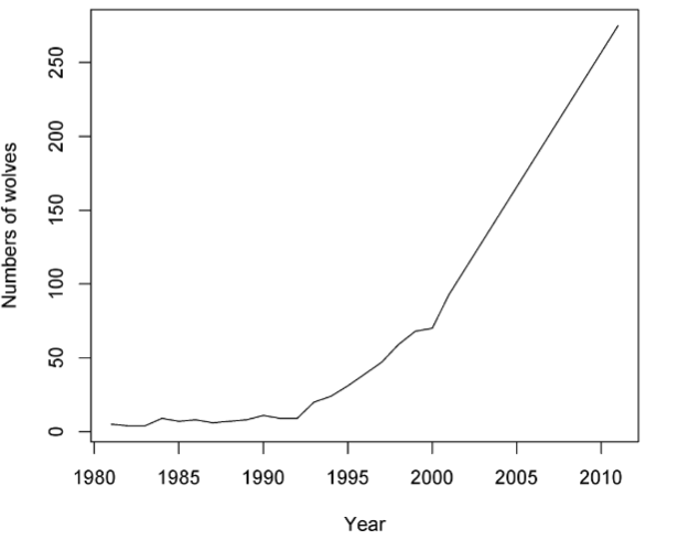
Case Study: growth in Scandanavian wolf populations (and bottleneck)

• A previously unknown pack of <10 wolves was discovered in 1983

• Without any external changes in management, the population began increasing in 1991 by 29% annually

• Genetic data suggest there were only two founding wolves, probably from Russia or Finland (not a relic population)

Case Study: human population growth (including Von Foerster doomsday prediction)

• Until the last 20 years or so, it looked exponential, with no end in sight

• Von Foerster thought the population would go to infinity on Nov 13 2026

• He determined that the population growth rate was actually greater than exponential -- r is increasing

Case Study: Malthus studied growth in England (density dependent) and the US (more density independent)

Malthus thought that higher growth rates in the U.S. were due to better living conditions, he also thought that England’s fewer resources caused a lower growth rate and less morals

Case Study: Temperature affects r and K in Moina

Temperature affects little r

As temp increases, little r increases

K has highest value at **intermediate** temp

competition

a reduction in resource acquisition rate (feeding, foraging, parasitism, nutrient uptake) due to the action or presence of another individual that seeks to acquire the same resources

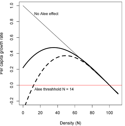
allee effects

mechanisms arise from cooperation or facilitation among individuals in the species, such that they do a bit better in groups.

Examples of such cooperative behaviors include better mate finding, environmental conditioning, and group defense against predators

intraspecific competition

competition within species

interspecific competition

competition between different species

K

carrying capacity

minimum viable population size

Smallest population that can be predicted to have some probability (e.g., 95%) chance of persisting for some number of years (e.g., 100 or 1000 years)

environmental stochasticity

this when there are random environmental fluctuations affect the average birth and/or death rates, in turn causing variation in the population growth rate

demographic stochasticity

variation in population growth rates arising from differences among individuals in survival and reproduction

time lags

occur when population growth rates are determined not by the density at the present time, but by the density at some other time.

One example is gestation time – when times are good, animals may mate, but the effects on density may not occur until the offspring are born and achieve some size

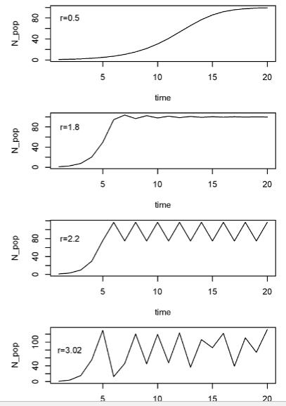
chaos

time lags can cause oscillations. As the lag or r increases, the population will first have damped oscillations, then fixed oscillations, then 2-point oscillations, then

CHAOS

not random

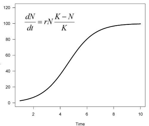
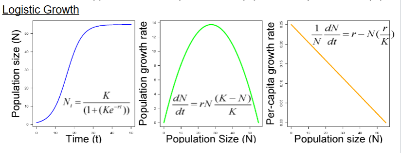
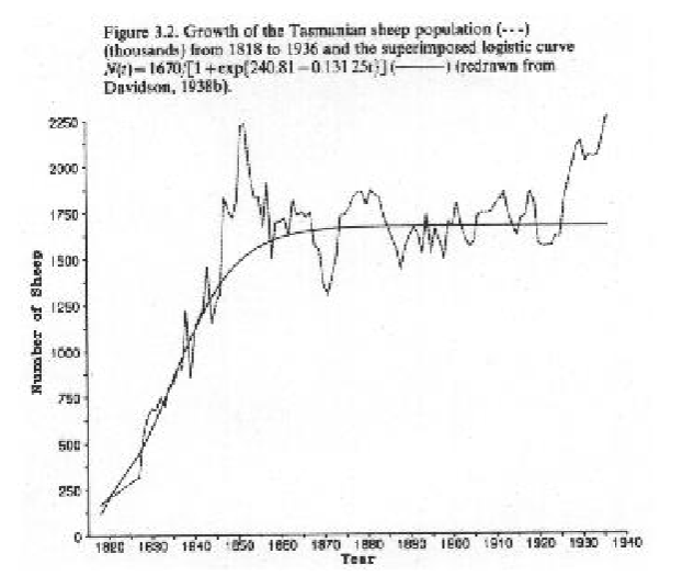
Logistic growth does occur in nature

example of barnacles and sheep

Assumptions of logistic growth (constant r and K)

In real life:

The carrying capacity is not constant (environmental stochasticity). Birth and death rates (or r and R) do not change in a linear way with density

Most populations are affected by both

density-dependent and density-independent

Logistic growth in Drosophila

Example of how genetics or environment can affect competition , r and the carrying capacity (K).

MVP example from Bighorn Sheep

Populations with fewer than 50 individuals went extinct within 50 years

Lionfish and density independence

Benkwitt transplanted lionfish onto 6 reefs at 6 different densities. I also established and maintained 4 reefs with 0 lionfish as controls. All treatments were started within a 2-week period.

Individual growth in length declined linearly with increasing lionfish density, while growth in mass declined exponentially with increasing density. There was no evidence, however, for density-dependence in recruitment, immigration, or loss (mortality plus emigration) of invasive lionfish. The observed density-dependent growth rates may have implications for which native species are susceptible to lionfish predation, as the size and type of prey that lionfish consume is directly related to their body size.

density vague

suggests that there is some average population level around which a regulated population fluctuates. As the populations is perturbed further from this average level, density becomes more important in “pushing” the population back towards the average.

How much it fluctuates depends on the relative importance of density dependent and independent factors.

density vagueness concept

It reveals that ALL

natural populations are really controlled by both density

dependent and density independent factors

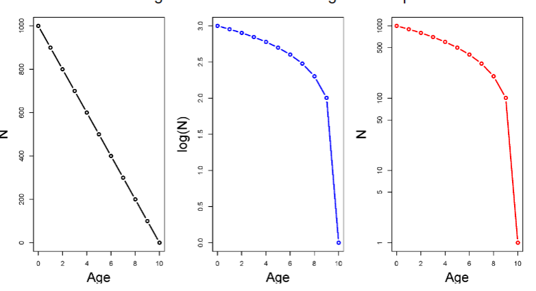
lx or survivorship

survivorship from the beginning number

AKA #survived/# we started of with

cohort life table

are constructed by following an even age group (such as all the eggs in nests from one year) throughout their entire life. At any point in time, they are all the same age

show the probability of death of people from a given cohort

px or age specific survival

tells us which portion survives in the next time period

Density dependence vs. density independence is resolved by density vague

ALL natural populations are really controlled by both density-dependent and density independent factors

Y-axis for survivorship curves

the y axis may be plotted in several different ways. For example, the y axis may be actual numbers of individuals or proportions (this won’t affect the shape of the curve). Or, even more confusing, the y axis may be either log transformed or on a log scale -- this does change the shape!

Sex-specific differences in survival

Females tend to have higher mortality during

childbirth years. However, females tend to live longer

Eisenberg’s snails

He conducted a simple experiment in 1966 to see if snails in a pond exhibited density dependent growth and to determine what factors might limit the snail population growth (e.g., competition or predation

food didn’t affect lx but did affect bx

Erickson’s dinosaurs

show type I survivorship curve

Type I survivorship

exhibit high juvenile survival and are common for mammals

Type 2 survivorship

is constant probability of death (or survival) across age classes.

ex: birds

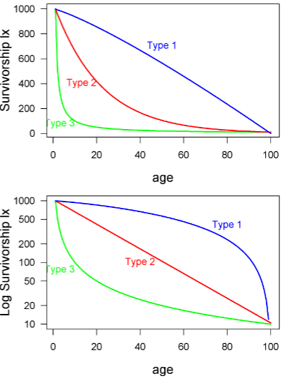
Type 3 survivorship

at younger age, higher chance of dying

ex: fish, insects

mx

average births per individual age x

lxmx

The lxmx for each age group tells us the reproductive contribution of each age group, weighted by the probably of surviving to reproduce

R0

sum of lxmx

If greater than 1= growing

If less than 1= decreasing

generation time

= mean age of mothers at the time of their mean daughter’s birth

= summation xlxmx / R0

stable age distribution

using R0 assumes that the population has achieved a stable age distribution.

Another way of determining R0

the sum of lxmx

Life table vs. population projection

Life tables do not have densities or abundances (N’s)!

However, we can now take this life table and predict what will happen to any given population through time. This is a population projection.

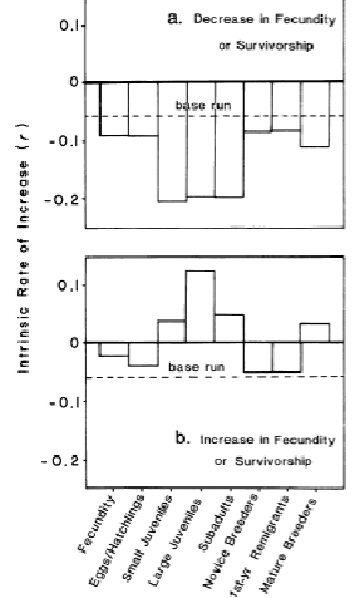
sensitivity

the slopes of these lines (in sensitivity analyses) are a measure of the sensitivity of the population growth to values in the life table

sensitivity analyses

This is used to see which birth or death rates most affect the overall population growth rate

How you get the stable age distribution and how it relates to R0

stable age distribution: the proportion of the population occupied by each age class remains constant. This pattern is seen in populations with a declining birth rate and a low death rate.

if either r or R0 is constant, then you have exponential growth IF you are at the stable age distribution

Remember how r and R0 differ

Increasing; r is constant and positive; R0 is greater than one

Decreasing: r is negative; R0 is less than one

Converting between r and R0

r = ln(R0)/G

R0 = e^rG

Emperor geese, sensitivity analyses

We need R0 greater than 1. So, the only way we could get that would be to increase juvenile survival or to increase adult egg production

R0 is most sensitive to changes in juvenile survival

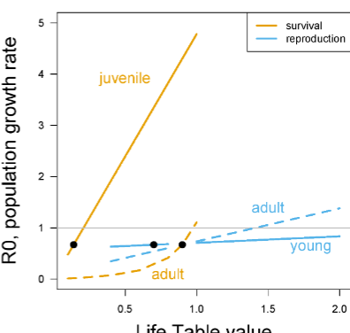
Sea turtles, sensitivity analyses

Looking at the bottom graph, the best thing is to save large juveniles

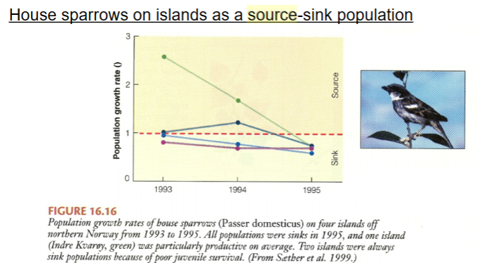
sink population

a net import of individuals (immigration > emigration)

source population

a net export of individuals (emigration > immigration)

rescue effect

The populations in some patches are maintained only through continuous migration, otherwise the population would go extinct. In effect, these sink populations are being continuously “rescued” from extinction

Regional population

a group of local populations

metapopulation

is a group of several local populations that are linked by immigration and extinction

Local population

make up a metapopulation

Going from studying population numbers to numbers of populations

instead of births and deaths, we focus on colonization of new patches and extinctions of patches

When do you have a metapopulation

at intermediate dispersal among patches)

Probabilities of patch colonization and extinction in b-d form

dP/dt= cp(1-P)-Ep

this equation states the growth tare of local populations can be determined by colonization’s and extinctions

Local vs. regional population persistence with number of local populations

the probability of regional persistence for one year is (1 - the probability that both patches go extinct during the year)

Persistence of x patches = 1 – (e)^x

Potential role of corridors

a way to link local populations

Hanski’s butterflies in dry meadows on islands

Some of the first work on metapopulations was by Ilka Hanski, who studied butterfly populations on dry meadows on islands near Finland

Populations in these patches aren’t static or unchanging. Instead, some populations may increase in size, while others decline. Some may go extinct, while others are being colonized

Sparrows on four island demonstrating sources and sinks

Sparrow populations on four islands off the coast of Norway, with migration among the islands. All islands maintained relatively constant number across the three years of this study, with migration from source populations “rescuing” sinks. The graph shows that some islands are more productive that others, acting as sources in good years. But, in severe years, all populations are sinks

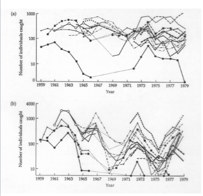
Beetles in the Netherlands showing rescue effects

For the beetle Pterostichus versicolor, the abundances vary asynchronously and there were no extinctions over the 21 years.

For the beetle, Calathus melanocephalus, populations varied somewhat synchronously, leading to occasional local extinctions.