Data Visualization in the Social Sciences - Midterm

Flashcards covering key vocabulary and concepts from the lecture on Distributions and Histograms in Social Sciences.

Column/bar chart

A chart that presents the frequency of categorical variables.

Histogram

A chart created without converting data to categories; it requires selecting a size for the 'bins'.

Bar height (Histogram)

Number of observations in bin.

Bar width (Histogram)

Range of values of the continuous variable.

Clustered column charts

These charts visualize group differences in categorical variables.

Patterns of Distributions

Bell-shaped or Normal: symmetric, unimodal; U-shaped: symmetric, bimodal; Right-Skewed / Positive: long right tail; Left-Skewed / Negative: long left tail

Visually Identifying Normal Distribution

Symmetry and Fit of a normal bell curve

Mathematically Identifying Normal Distribution

Calculate skewness, Skewness value of 0 is perfectly normal, Large absolute value of skewness indicates more skew, Test for normality

Describing Continuous Data: Descriptive Statistics

Where is the center? Central Tendency, How spread out? Variability

Arithmetic Mean

(Sum of observed scores) divided by (number of scores)

Standard Deviation

Shows how closely scores cluster around the mean.

Median

The middle score; the score that divides the ranked data in half

Quartiles

Values that cut the distribution in quarters (fourths).

Interquartile Range (IQR)

Q3-Q1

Box and Whisker Plot Benchmarks

Min, Q1, Median, Q3, Max

Mode

Most frequently occurring score.

Range

Highest score – lowest score

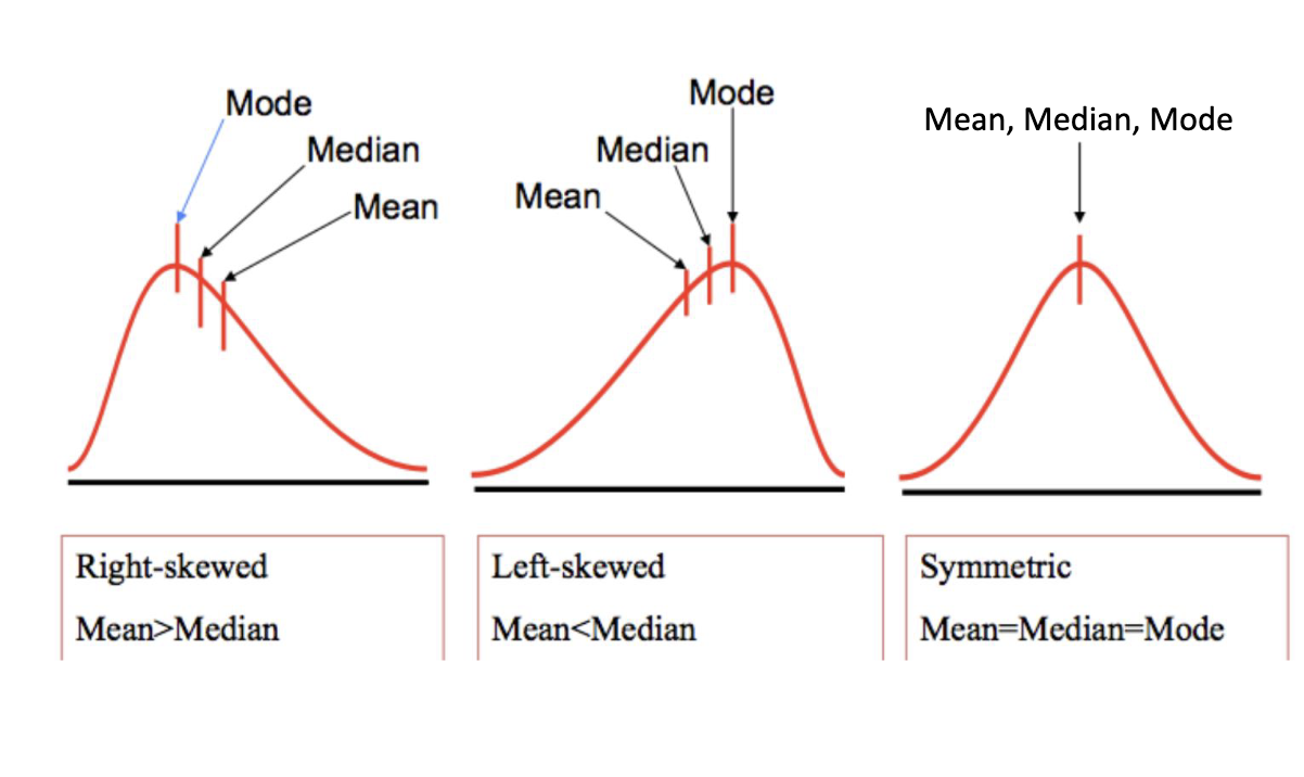
Distributions and Measures of Central Tendency

Symmetric: Mean=Median=Mode; Right-skewed: Mean>Median; Left-skewed: Mean<Median

Effect Size

the magnitude or ‘strength’ of the association between the predictor variable and outcome variable

Sampling Distribution

the distribution of sample statistics from a large number of random samples

Sampling error

differences between the sample statistics and things we want to measure in the population due to random chance

Standard error

measures how much we expect sample statistics to vary from one sample to the next

Qualitative

information in written form that are no summarized; written descriptions. Open ended questions could result in written response with much detail

Quantitative

information summarized (quantified) in numbers (values) or standard categories (groups). This limits the detail that is gathered but allows the data to be summarized.

Continuous Data

(numbers) has values that indicate quantity or amount (e.g. years, months, days)

Main effect

the effect of one predictor variable on one outcome variable. The two variables are either related (there is a main effect) or are not related (no main effect).

Relationship Between Predictor Variables

When there are two or more predictor variables, they either share an additive relationship or they interact.

Collapse the Data over Variable A

Ignore the levels of variable A

Categorical Variables are visually represented by

column/bar charts which present the frequency of categorical variables.

Bar Height of a Histogram

represents number of observations in bin

Bar Width of a Histogram

is a range of values of the continuous variable

Why do you need to be careful with bin width?

Very large bin=loss of detail
Very all bin=loss of context in data interpretation & is very messy/cluttered

You can think of histograms as…

imahine each person is a brick, and you are stacking the bricks into each “bin” based on hourly wagess

Right-Skewed/Positive

long right tail

Left-Skewed/Negative

long left tail

How do I tell if a distribution is normal or skewed?

1. Visually (symmetry & fit of normal bell curve)

2. Mathematically: calculate skewness (normal distribution would have a skewness value of 0 & large absolute value of skewness indicates more skew)

3. Test for normality

What does a normal distribution tell us?

• more naturally occurring phenomenons in many real-world situations, where most observations cluster around the mean with symmetric tails.

EX:

What does a skewed distribution tell us?

distributions can become skewed when there is a minimum and no maximum value or run into a maximum or minimum possible value
EX: hourly wage & number of children per adult(positive skew), Grades in 12Y (negatively skewed)

Descriptive Stats for “Where is the center?”

Central Tendency:
- Mean (average)
- Median (middle value)
- Mode (most frequent)

Descriptive Stats for “How spread out?”

Variability:

• Standard Deviation

• Interquartile Range

• Range

To describe normal distributions use the

mean & standard deviation (always report the standard deviation when reporting the mean)

Standard deviation describes

how closely scores cluster around the mean (large SD means that there is more spread)

Steps for calculating standard deviation

1. subtract the mean from each score (find the differences)

2. square the differences (get rid of negative numbers)

3. Sum the squares

4. divide by n-1

5. Squareroot

To describe skewed distributions use the

median & interquartile range (always report the IQR when reporting the median)
median is less sensitive to outliers than the mean

Calculate IQR

1. Calculate the mean

2. Calculate the median of the bottom half (Q1)

3. Calculate the median of the top half (Q3)

4. Q3-Q1

Box Plots represent…

Min, Q1, Median, Q3, and Max
They also make it easier to visually compare distributions between groups

Mode

most frequently occurring score
There can be two (or more) modes; bi-modal

Range

Highest score-lowest score

Visual representation of distributions and measures of central tendency

Main Effects

• 1 outcome & 1 predictor

• Associated (Related): outcome is different by levels of predictor

• Independent (not related): outcome is same by levels of predictor

For bimodal distributions…

the measures of central tendency and variability are not going to accurately describe the data

Relationship between predictor variables

• 1 outcome & 2+ predictors

• Interaction: effect of one predictor is different depending on the level of other predictor(s)

• Additive: effect of one predictor is the same regardless of the level of the other predictor(s)

Effect Size

the magnitude or ‘strength’ of the association between the predictor variable and outcome variable

It is based on the difference between the means and the amount of variability

If the variability is the same, but one pair of means are farther apart

• there is less overlap

• there is a bigger effect size

• it will be easier to detect

If the mean differences are the same, but one pair has smaller variability, then

• there is less overlap

• there is a bigger effect size

• it will be easier to detect

Sampling distribution

the distribution of sample statistics from a large number of random samples
ex: distribution of average family income form multiple randome samples of 1,500 families in the U.S.

Sampling error

• differences between the sample statistics and things we want to measure in the population due to random chance

• increasing sample size decreases sampling error

  • the sampling distribution with n=20 (compared to n=10) has less variation, and more closely resembles a normal distribution

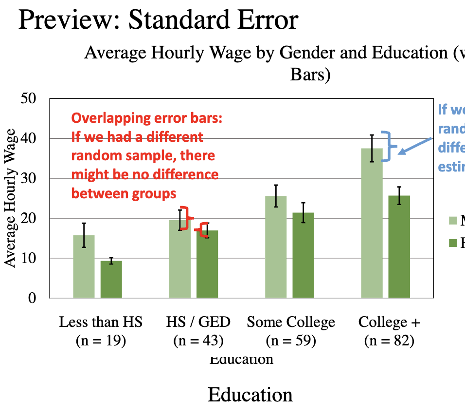
Standard error

measures how much we expect sample statistics to vary from one sample to the next
it is also the difference between a sample and the population due to random chance

Overlapping error bars

if we had a different random sample, there might be no difference between group

Population of interest

• the entire group or situation you are interested in

• it is often not feasible to gather data on the entire population

Sample

• Each sample is an estimate of the underlying population

• No two samples will be the same due to random sampling error

Representative Samples

• attempt to have the sample look just like the population

• every member of the population has an equal chance of being selected

Non-Representative Samples

• Systematically different from the population

Stratified Random Sampling

• List every member of population

• Identify subgroups

• Randomly select proportionally from subgroups

Non-Representative Sample:

voluntary response sample

convenience sample

quota sample

Standard Normal Distribution

• The area under the curve is 1 or 100%

• we know the proportion of a population in a range of values based on the mean and standard deviation of a symmetric, bell-shaped distribution

Why do we take samples?

to estimate a population

How do we know if our sample is close estimate of the population?

Because sampling distributions are normally distributed

What does the Standard Normal Distribution tell us?

68% of the population is within ±1 SD of the Mean (most sample means will lie reasonably close to the population mean and that is within this context)

Margin of Error

how much the sample mean differs from the true value in the population

If the margin of error overlap on the y-axis

we can conclude that there is no evidence of a significant difference

“within the margin of error

If the margins of error do not overlap on the y-axis,

we can conclude that there is likely evidence of a significant difference
“outside the margin of error”

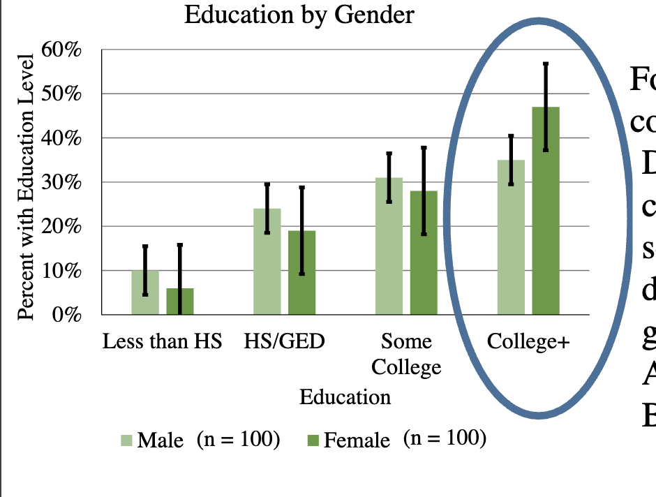
For those with college education, does the % with college education seem significantly different by gender?

No

For categorical variables…

describe: percentages
Margin of error: based on sample size (as sample size increases, the margin of error decreases)

Continuous Variables

Describe: mean or median

Margin of error: based on sample size and variability
Can be represented using: Standard error of the mean (SEM) or Confidence Interval (usually 95%)

Standard Error of the Mean (SEM)

SD/Sqrt(n)

If the mean increases, the SEM

stays the same

Confidence Interval (CI)

the interval within which the population parameter is believed to be

Confidence level

the probability that the CI contains the parameter
multiple the SEM to reach the desired confidence interval

Margin of Error

z* value x SEM

Calculate a 95% confidence interval

1. calculate the standard error of the mean

2. calculate the margin of error

3. confidence interval is mean± margin of error
   mean-1.96(SD/sqrt(n))

The standard deviation will always be___ than the standard error of the mean

greater than

The standard error of the mean will always be ____than the 95% confidence interval

less than

How big of a sample do I need to be confident that it is similar to the population?

It depends…because categorical variables focus on the sample size only but continuous variables also take variability into consideration

How far apart do two samples means need to be before I can conclude that they are really different?

If the means fall outside of each other’s confidence intervals then they are likely to be samples drawn from different

Science is..

• determining if there are relationships between variables

• making comparisons between samples

• while accounting for error

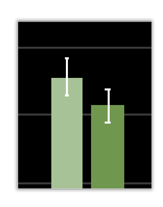
Visual reasoning with error bars

• error bars show the likely range for population parameter (mean or proportion)

• If the error bars overlap, then the samples may be from the same population

Null Hypothesis

prediction that there is no difference
cannot ‘prove it’, but we can fail to disprove it

Research hypothesis

the prediction we’re interested in testing; we require strong evidence to support the hypothesis
HYPOTHESES MUST BE MUTUALLY EXCLUSIVE

HYPOTHESES MUST BE MUTUALLY EXCLUSIVE (does not overlap with 1a and 1b); if

• Hypothesis 1a: Average income is the same for men and women.

• Hypothesis 1b: Average income is greater for men than women.

Then 1c is?

Average income is greater for women than men.

T-test/t-statistic

quantifies the difference between the group means, taking into account both variability and the sample size

Small t statistic (<2)

indicates that there is no evidence that the groups are different for this outcome

Large t statistic (>2)

indicates that the groups are likely to be truly different for the outcome

p-value

• a number between 0 and 1

• the probability of finding the t from our samples if there is really no difference between the groups

Larger t → smaller p-value

larger inferential statistic → smaller probability that there is no difference
if the p-value is really small (usually p<0.05), its very unlikely the group difference is due to chance

p<0.05

• reject H0

• statistically significant

• a real relationship

p>/= 0.05

• fail to reject H0

• not statistically significant

• no evidence of a relationship

What does a larger relationship mean?

A “larger relationship” means that the effect size or how distinct the groups are so, with less variability and more similar means=> stronger relationship

Categorical (outcome) x categorical (predictor) uses what function to relate the variables

chi-square

continous (outcome) x categorical (predictor) uses what function to relate the variables

t-test & mean and s.d. to describe the relationship