EMF final

A1

Linearity in parameters a and B, ensures OLS formulas are valid

A2

Random sample, each observation drawn independently

A3

Sample variation, no perfect collinearity, Var(x) =0

A4

Zero conditional mean of errors, E(u|x) = 0, the unobserved factors must be uncorrelated with x, ensures OLS estimators are unbiased

A5

Homoscedasticity, variance of the error terms must be constant Var(u|x) = sigma²

Unbiased

If on average it gives the true value of the parameter

E(a^) = a and E(B^) = B

A1,A2,A3,A4 have to hold

if E(B^) = B the difference is the bias

Efficiency

OLS is efficient if it has the smallest variance, means the estimates are most tightly clustered around the true value

A1,A2,A3,A4,A5 have to hold

TSS

SUM (Y - MU Y)², Total variation

ESS

SUM (Y^ - MU Y)², Variation explained by model

RSS

SUM (Y - Y^)², Variation not explained by model

A6

Normality, needed for hypothesis testing, the population error u is independent of the explanatory variables and normally distributed

u ~ N(0, sigma²)

Breusch-Pagan test

Test for homoscedasticity

Estimate normal regression

Obtain and square the error term and create new regression

u² = g0 + g1×1 + g2×2 + e

Use F-test, H0: g1=g2=0 is homoscedasticity

R² adjusted

1 - (RSS/(n-k-1)) / (TSS/(n-1))

F-test

((RSSr - RSSur) / q) / (RSSur / (n - k - 1))

F-test R²

((Rur² - Rr²) / q) / ((1 - Rur²) / (n - k - 1))

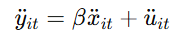
First Differences theory

yit = a + Bxit + ai + uit

ai is time-invariant unobserved effect

if ai is correlated with xit, OLS gives biased estimates

solve by subtracting previous period from current period

yit - yit-1 = B(xit - xit-1) + (uit - uit-1)

dyit = Bdxit + duit

key is ai - ai = 0 the unobserved time-invariant factor disappears

Fixed Effects Theory

yit = a + Bxit + ai + uit

ai is time-invariant unobserved effect

if ai is correlated with xit, OLS gives biased estimates

Solving this by removing ai through within transformation, subtracting each unit’s mean from its observations

yit - MU yi = B(xit - MU xi) + (uit - MU ui)

ai cancels out because ai - ai = 0

Random Effect theory

yit = a + Bxit + ai + uit

ai is time-invariant unobserved effect

if ai is correlated with xit, OLS gives biased estimates

keep ai in the model but treat as random variable, part of the error term (or just in the model) and assumes it is uncorrelated with explanatory variables

Cov(xit, ai) = 0

eit = ai + uit

yit = a + Bxit + eit

Use Generalized Least Squares to account for two components in the error term

Choosing between RE and FE

Hausman test

If the difference between FE and RE estimates is small, RE is likely valid and more efficient

If the difference is large, ai is correlated with xit and FE should be used

Endogeneity cases

Omitting relevant variables, excluding important factors due to data limitation or bad choice of model

Simultaneity, one ore more of the explanatory variables is jointly determined with y

Measurement error, one or more of the explanatory variables is measured with error

Instrumental Variables theory

Introducing a third variable z that helps isolate the causal effect x on y 

Two key conditions:

• Relevance: Cov(z,x) = 0, z is correlated with the endogenous regressor x

• Exogeneity: Cov(z,u) = 0, z is uncorrelated with the error term u

IV estimator is: Biv = Cov(z,y)/Cov(z,x)

Two-Stage Least Squares to estimate IV

Stage 1: predict x using the instrument

• xi = sigma + gzi + vi (all other independent variables)

• Gives xi^ the part of x explained by z

Stage 2: regress y on x^

• yi = a + Bxi^ + ui

DiD theory

Causal inference method used when we have data before and after a treatment

We compare changes over time in treatment and control group

yit = a +BDi + gPostt + sigma(Di x Postt) + uit

Di is dummy with 1 if unit is treatment group

Postt is dummy with 1 after treatment

gamma is the DiD estimator, the causal effect of the treatment

DiD removes both pre-existing differences and time trends

RDD theory

Causal inference method used when treatment is assigned based on a cutoff in a continuous variable

Units just below and just above the cutoff are assumed to be very similar, except one group received treatment, allows to estimate causal effect right at the cutoff

yi = a + rhoDi + f(Ri) + ui

Di is treatment indicator

rho is treatment effect at the cutoff

Ri is running variable

f(Ri) is smooth function of the running variable

Assumption: all other factors affecting y change smoothly around the cutoff

Logit and Probit intuition

The idea is that instead of modeling the probability directly as a linear function (LPM) we model an unobserved latent variable y

As x increases the probability P(y=1|x) changes non-linearly

The models capture the realistic idea that probabilities flatten out as they approach 0

Omitted variable bias

True Model y = a + B1X1 + B2X2 + B3X3 + u

Used model y = a +B1X1 + B2X2 + v

E(B1~) = B1 + B3sigma~

determine if sigma and B3 are positive or negative

Clustering by firm, type of dependence and consequence

Clustering by firm corrects time dependence

Clustering by time period would correct for cross-sectional dependence

Not clustering would leed to lower se which inflate t statistic