Data analysis

Observed variable , Response variable, Dependent variable, Explained variable, Outcome variable

The variable that we aim to model or predict, typically denoted by y. It depends on the input variables.

Fit parameters, Regression coefficients

The unknown parameters of the model (usually denoted by Greek letters like theta) that are estimated from the data during model fitting.

Explanatory variable, Regressor, Independent variable, Covariate, Predictor

They are the inputs of the model, typically denoted by x.

Variables that are used to explain or predict the observed variable.

Noise, Error term, Disturbance term

It represents random fluctuations or measurement errors, usually denoted epsilon.

The part of the variation in the observed variable that is not explained by the model.

Design matrix, Predictor variable matrix

A matrix X that contains all the predictor values for the observations, structured so that each row corresponds to one observation and each column to one predictor.

linear ordinary least-squares (OLS)

Statistical method used to estimate the parameters of a linear regression model by minimizing the residual sum of squares (RSS) between observed responses and model predictions. All observations are treated equally; there is no weighting

Residual sum of squares (RSS) , Objective function, Chi² function, loss function, cost function

A function that quantifies the discrepancy between the observed data and the model predictions.

normal equations

They provide a direct (analytical) way to compute the best-fit parameters for a linear model.

R-style formulae

a concise and expressive syntax used to specify statistical models, originally from the R programming language

f.e. y ~ x₁ + x₂

so y= θ₀ + θ₁x₁ + θ₂x₂ + ε

Homoscedascity

Refers to the behavior of the variance of the error terms in a regression model.

The error terms have constant variance across all levels of the explanatory variables.

This is a core assumption of Ordinary Least-Squares (OLS) regression.

heteroscedascity

Refer to the behavior of the variance of the error terms (or residuals) in a regression model.

The error variance varies with the level of one or more explanatory variables.

Plot residuals vs. fitted values; a fan or funnel shape suggests heteroscedasticity.

expected value

The average value when repeating the experiment many many times

Residuals

Residuals are the differences between the observed values and the predicted values from the model.

Small residuals → good fit; large residuals → poor fit or model misspecification.

Predicted responses

These are the model’s best estimates of the observed variable under the assumed model.

Predicted responses are the fitted values.

t-value

The number of standard errors the fit parameter is away from zero.

A large absolute value of t suggests that the corresponding variable is statistically significant.

(A small t-value (close to 0) suggests that the coefficient may be zero, and thus the variable might not contribute meaningfully to the model.)

confidence interval

A confidence interval for a parameter (e.g. θ) is a range of values, derived from the data, that is likely to contain the true value of the parameter with a specified probability, assuming the model and its assumptions are correct.

For example, a 95% confidence interval for θ means:

“If we repeated the experiment many times, and each time constructed a 95% confidence interval, then about 95% of those intervals would contain the true value of θ.”

The more data you gather, the more confident you are in the estimated fit parameters

confidence level

The confidence level is the probability that the confidence interval procedure will produce an interval that contains the true parameter value. It is typically expressed as a percentage:

• 95% confidence level → 5% of intervals may not contain the true value.

This level defines the width of the confidence interval: higher confidence → wider interval.

Note: A 95% confidence level corresponds to a split in two equal parts: 2.5% at either side of the interval .

joint confidence ellipsoid

It shows where the true values of several fit parameters are likely to lie together, taking into account their uncertainties and how they are correlated. It's like a multi-parameter version of a confidence interval.

Coefficient of determination (R²)

Is a statistical measure used to assess the goodness of fit of a regression model. It quantifies how much of the variance in the observed data is explained by the model.

R²=1: Perfect fit

An R² of 0.85 means that 85% of the variation in the observed variable is explained by the model.

Adjusted coefficient of determination

It tells how well the model explains the data, but also corrects for the number of predictors used. It only increases if adding a new variable actually improves the model. Don’t use it for model selection.

mean response, fitted value of the response, expected value of the response

The value you'd expect if you repeated the measurement many times under the same conditions.

t-multiplier

It is a value from the Student’s t-distribution used to construct confidence intervals.

α/2 quantile of the student’s t-distribution with N-K degrees of freedom

N= number of observations

K= number of fit parameters

multicollinearity

When one predictor can be written as a lineair combination of the other.

unidentifiability

It happens when the determinant is zero, so it’s impossible to uniquely determine the values of some fit parameters.

ill-conditioning

How sensitive the solution of a system of equations is to small changes in the input data. Thus the situation where the design matrix X of a regression model is numerically unstable

condition number

A numerical indicator that measures how ill-conditioned a matrix is. That is, how sensitive the solution of a system of equations is to small changes in the input data.

recentering

Means subtracting the mean from the responses and design matrix. Is applied when the values of one regressor is order of magnitude larger than those of another regressor.

unit-scaling or standardizing

means adjusting variables so they all have similar ranges, by subtracting the mean and dividing by the standard deviation for the responses and design matrix.

High-leverage points

Outliers in the x-direction, that can strongly influence the regression fit. They may or may not be outliers in y.

CHAPTER 2

consistent estimator

Is an estimated parameter that gets closer to the true parameter value as the sample size increases.

Weighted least-squares (WLS)

version of linear regression where each data point is given a weight, so points with more reliable measurements have more influence on the fit.

It's especially useful when the data show heteroscedasticity (non-constant noise levels).

Feasible Weighted Least-Squares

is a two-step version of WLS used when the error variances are unknown.

First, you estimate the error pattern, then use those estimates to assign weights and perform a weighted regression.

CHAPTER 3

nonlinear least-squares

is a fitting method used when the model depends nonlinearly on its parameters.

But unlike linear least-squares, it requires iterative algorithms to find the best-fit parameters.

expectation surface

It shows what the model expects on average, without noise, over the entire input space.

is the surface formed by the mean predicted values (or expected values) of the response variable across different combinations of predictor values.

a 100(1-α)% confidence region

Is the area (or volume) in parameter space where the true values of the parameters are expected to lie with (1−α)×100% confidence, based on the data and model.

For example, a 95% confidence region means we expect the true parameters to be inside that region 95% of the time in repeated experiments.

CHAPTER 5

Least trimmed squares (least trimmed sum of squares)

is a robust regression method that fits a model by minimizing the sum of the smallest squared residuals, ignoring the largest ones

(alters cost function so it can better deal with outliers)

least trimmed sum of absolute deviations

is a robust regression method that fits a model by minimizing the sum of the smallest absolute residuals, rather than squared ones.

Least quantile regression

Is a robust regression method that minimizes the median of the squared residuals, instead of minimizing the mean

(alters cost function so it can better deal with outliers)

Huber’s method

Rather than computing the square of the residual, we could use another function of the residual which would be less sensitive to outliers

(alters cost function so it can better deal with outliers)

CHAPTER 6

AIC score

Is a model selection metric used to compare statistical models. It balances model fit with model complexity, penalizing models with more parameters. It is used for comparing models on the same dataset.Lower AIC = better model (relative to others).

Likelihood

the probability of observing the data given specific parameter values

“we assume that observations are“ independent and identically distributed (i.i.d.).

Means that all data points are drawn from the same probability distribution and are statistically independent of each other.

method of maximum-likelihood

estimates model parameters by finding the values that maximize the likelihood

Akaike delta-score

difference in AIC values between a given model and the best (lowest-AIC) model.

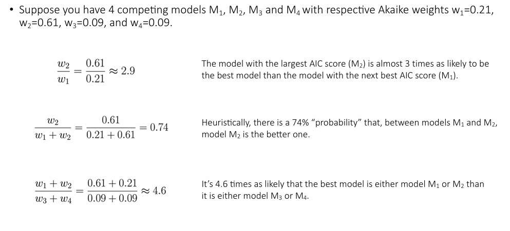
Akaike weight

represent the relative likelihood of each model being the best among a set, given the data.

Cross-validation

is a technique to assess how well a model generalizes to new, unseen data. It works by splitting the data into parts: the model is trained on some parts and tested on the remaining part, repeating this process multiple times to get a reliable estimate of prediction performance.

Test error (also called generalization error)

is the error a model makes on new, unseen data. It reflects how well the model generalizes beyond the training data

K-fold cross-validation

is a method to estimate a model’s test error by splitting the data into K equal parts (folds). The model is trained on K−1 folds and tested on the remaining fold, repeating this K times so every fold is used once for testing. The average test error across all folds gives a reliable performance estimate.

Leave-one-out cross-validation

is a special case of K-fold cross-validation where K equals the number of data points. Each time, the model is trained on all data except one point, which is used for testing. This is repeated for every point, giving a nearly unbiased estimate of test error, but at high computational cost.

CHAPTER 7

ridge regression / Thikonov regularization

type of linear regression that adds a penalty term to the loss function to shrink the regression coefficients. This helps prevent overfitting and reduces the impact of multicollinearity by discouraging large coefficient values.

Regularization term or penalty term (λθ’θ)

is an extra part added to a model’s loss function to penalize large or complex parameter values. It helps prevent overfitting by encouraging simpler models.

λ penalty parameter / regularization parameter

controls how strongly the regularization term affects the model. A larger λ puts more penalty on large coefficients, leading to a simpler model, while a smaller λ keeps the fit closer to ordinary least squares.

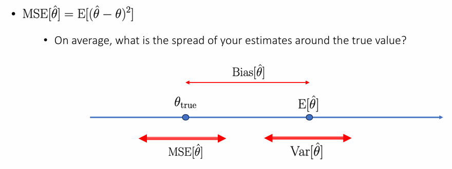
Mean Squared Error

calculates the average of the squared differences between predicted and actual values.

Ridge trace

A ridge trace is a plot that shows how the regression coefficients change as the ridge penalty λ\lambdaλ increases.

LASSO (Least Absolute Shrinkage and Selection Operator)

a regression method that adds a penalty on the absolute values of the coefficients. It not only shrinks coefficients like ridge regression but can also set some to zero, effectively performing variable selection.

CHAPTER 8

non-parametric resampling

method that generates new datasets by randomly sampling from the observed data, without assuming any underlying distribution.

non-parametric bootstrapping

resampling method where you repeatedly draw random samples with replacement from the original dataset to create many “new” datasets. (without assuming any specific data distribution.)

pairwise resampling OR random-x sampling

a type of bootstrap where you resample entire (x, y) pairs from the dataset.

This method preserves the relationship between inputs and outputs and is commonly used when both are considered random.

residual sampling or fixed x-sampling

is a non-parametric resampling method for regression where the predictor values are held fixed, and synthetic response values are generated by adding resampled residuals to the model's fitted values.

parametric bootstrap sampling

method where new datasets are generated by simulating from a specified probability model using the fitted parameters from the original data.

Percentile bootstrap interval

Build a confidence interval by taking the lower and upper percentiles from the sorted bootstrap estimates (e.g. 2.5% and 97.5% for a 95% interval).

A pivot

a quantity that has a distribution that does not depend on any unknowns.

bootstrap-t interval

A confidence interval made by standardizing bootstrap estimates using their standard errors, then using the percentiles of these t-like values to build the interval. It adjusts for both bias and variability.

Balanced bootstrap resampling

guarantees that each observation is selected equally often.

CHAPTER 9

Law of bayes

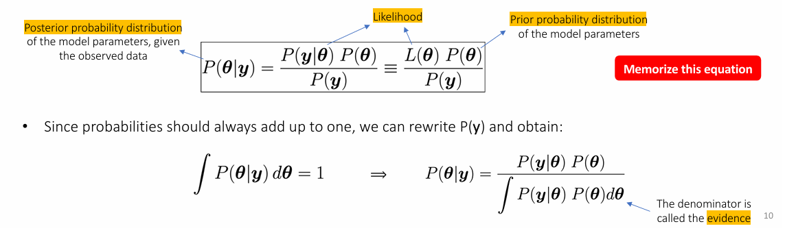
Posterior probability distribution

the probability of the parameters given the observed data

prior

our initial beliefs about the parameters before measuring the data

evidence

the total probability of the data, acting as a normalization constant

CHAPTER 10

conjugate prior and conjugate distributions

A prior is a conjugate prior for a given likelihood function, if the resulting posterior belongs to the same distribution family as the prior (Same distribution but with different parameters).

The prior and the posterior are called conjugate distributions.

hyperparameters

Settings that control the behavior of a model or method but are not learned from the data — they must be set before or tuned during training.

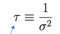
precision

It measures how tightly data or parameter estimates are concentrated — higher precision means lower uncertainty.

informative priors

If you have concrete information about a fit parameter, other than what the data is telling you, then the prior is the place where to include this information. Such priors are called informative priors.

uninformative priors

Quite often, you will not have any particularly useful prior information. In that case you would like to use a prior that is sufficiently vague so that you’re making only minimal assumptions

location parameter

A location parameter shifts the entire probability distribution left or right without changing its shape.

Scale parameter

Changing the scale parameter of a distribution stretches out the distribution

improper prior

Does not integrate to 1

proper prior

Does integrate to 1

Hyperprior

hyperprior = “a prior on a prior”

they have a probability distribution determined by another prior

CHAPTER 11

curse of dimensionality

If we have e.g. 5 model parameters (few...), and if we choose to evaluate the posterior in a rectangular grid of 100 points (not a lot!) in each of the 5 directions, we would need 1005 = 10’000’000’000 grid points. Unfeasible... This is called the curse of dimensionality

Normalization

Probability adds up to 1

Marginalisation

Marginalisation means summing or integrating out unwanted variables from a joint probability distribution to focus on the ones you care about

Expectation

the mean value of a parameter, given its posterior distribution

posterior predictive distribution

The distribution of possible future observations, based on the posterior distribution of the model’s parameters. It shows what new data might look like, given what we’ve learned from the current data.

Monte Carlo method

A computational method to sample an arbitrary probability distribution

cumulative distribution function

The CDF gives the probability that a random variable is less than or equal to a value x

Quantile function or percentile-point function

inverse cumulative function

acceptance-rejection method.

A way to generate random samples from a complex distribution by sampling from a simpler one and accepting or rejecting each sample based on a probability rule.

importance sampling

A technique to estimate expectations by sampling from an easier distribution and reweighting the samples to reflect the target distribution

Markov Chain Monte Carlo

a method that explores the sample space using a Markov chain. • Such a chain walks from one point xn to the next xn+1 in such a way that the chain spends more time in the more important regions (where the density f() is high).

a Markov chain has no memory