MM - Chapter 6: Lossless Compression Algorithms

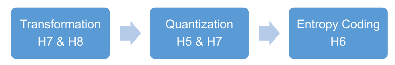
3 main steps of a compression scheme

Three main steps in a compression scheme

• Transform: the input data is transformed to a new representation that is easier or more efficient to compress.

• Quantization: we use a limited number of reconstruction levels (fewer than in the original signal) ➔ we may introduce loss of information

• Entropy Coding: we assign a codewords to each output level or symbol (forming a binary bitstream)

lossy vs lossless (kort)

If the compression and decompression processes induce no information loss, then the compression scheme is lossless; otherwise, it is lossy.

vb lossless: morse code

wat is entropy

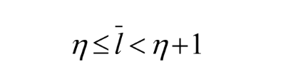
The entropy η is a weighted-sum of the symbols’ self-information log2​(1/pi​)

• hence it represents the average amount of information contained per symbol in the source S

The entropy η specifies the lower bound for the average number of bits to code each symbol in S, i.e.,

where l^(streep) is the average length (measured in bits) of the codewords produced by the encoder.

run length coding

• Memoryless Source: an information source that is independently distributed

  • value of current symbol does not depend on the values of the previously appeared symbols

• Instead of assuming memoryless source, Run-Length Coding (RLC) exploits memory present in the information source

• Rationale for RLC: if the information source has the property that symbols tend to form continuous groups, then such symbol and the length of the group can be coded

shannon-fano algorithm

top down approach

• Sort the symbols according to the frequency count of their occurrences.

• Recursively divide the symbols into two parts, each with approximately the same number of counts, until all parts contain only one symbol.

Other partitioning can lead to other coding trees

• potentially with other average codeword length

• huffman coding algorithm

• properties

bottom up approach

1. Initialization: put all symbols on a list sorted according to frequency

2. Repeat until the list has only one symbol left:

   • pick two symbols with the lowest frequency counts; form a Huffman subtree that has these two symbols as child nodes and create a parent node.

   • assign the sum of the children’s frequency counts to the parent and insert it into the list such that the order is maintained.

   • delete the children from the list.

3. Assign a codeword for each leaf based on the path from the root.

Unique Prefix Property: No Huffman code is a prefix of any other Huffman code → no ambiguity in decoding.

Optimality: minimum redundancy code - proved optimal for a given data model (i.e. a given, accurate, probability distribution):

• the two least frequent symbols will have the same length for their Huffman codes, differing only at the last bit.

• symbols that occur more frequently will have shorter Huffman codes than symbols that occur less frequently.

• the average code length for an information source S is strictly less than η + 1. Combined, we have:

  

extended huffman coding

• Motivation: All codewords in Huffman coding have integer bit lengths. It is wasteful when pi​ is very large and hence log2​(1/pi​) is close to 0

• Why not group several symbols together and assign a single codeword to the group as a whole?Extended Alphabet: For alphabet S = {s1, s2, ..., sn}, if k symbols are grouped together, then the extended alphabet is:

  

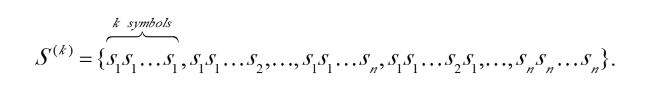
It can be proven that the average # of bits for each symbol is

An improvement over the original Huffman coding, but not much.

Problem: If k is relatively large (e.g., k ≥ 3), then for most practical applications where n ≫ 1, nk implies a huge symbol table, which is impractical

adaptive huffman coding

Statistics are gathered and updated dynamically as the data stream arrives

• Initial_code assigns symbols with some initially agreed upon codes, without any prior knowledge of the frequency counts

• update_tree constructs an Adaptive Huffman tree

• It basically does two things:

  • increments the frequency counts for the symbols (including any new ones)

  • updates the configuration of the tree

• The encoder and decoder must use exactly the same initial_code and update_tree routines

Notes on Adaptive Huffman Tree Updating

• Nodes are numbered in order from left to right, bottom to top. The numbers in parentheses indicates the count

• The tree must always maintain its sibling property, i.e., all nodes (internal and leaf) are arranged in the order of increasing counts

• If the sibling property is about to be violated, a swap procedure is invoked to update the tree by rearranging the nodes

• When a swap is necessary, the farthest node with count N is swapped with the node whose count has just been increased to N +1

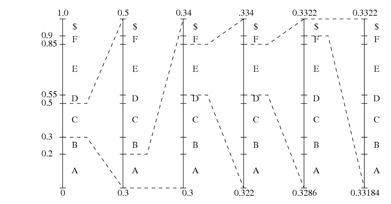
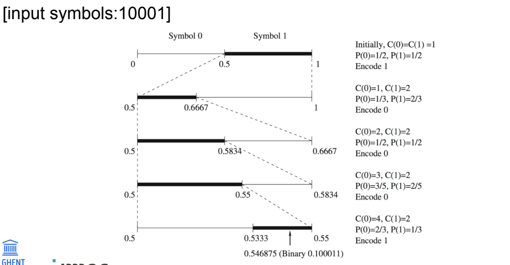
Arithmetic coding

• wat?

Arithmetic coding is a more modern coding method that usually out-performs Huffman coding

Huffman coding assigns each symbol a codeword which has an integral bit length. Arithmetic coding can treat the whole message as one unit.

A message is represented by a half-open interval [a, b) where a and b are real numbers between 0 and 1. Initially, the interval is [0, 1). When the message becomes longer, the length of the interval shortens and the number of bits needed to represent the interval increases.

enkele problemen en observaties bij arithmetic coding

The basic algorithm described in the last section has the following limitations that make its practical implementation infeasible:

• When it is used to code long sequences of symbols, the tag intervals shrink to a very small range. Representing these small intervals requires very high-precision numbers.

• The encoder will not produce any output codeword until the entire sequence is entered. Likewise, the decoder needs to have the codeword for the entire sequence of the input symbols before decoding.

Some observations:

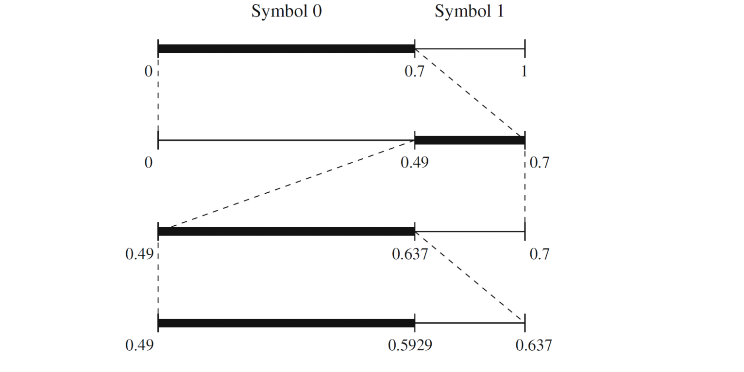
• Although the binary representations for the low, high, and any number within the small interval usually require many bits, they always have the same MSBs (Most Significant Bits).
  For example, 0.1000110 for 0.546875 (low), 0.1000111 for 0.554875 (high).

• Subsequent intervals will always stay within the current interval. Hence, we can output the common MSBs and remove them from subsequent considerations.

Verschillende soorten scaling bij arithmetic coding

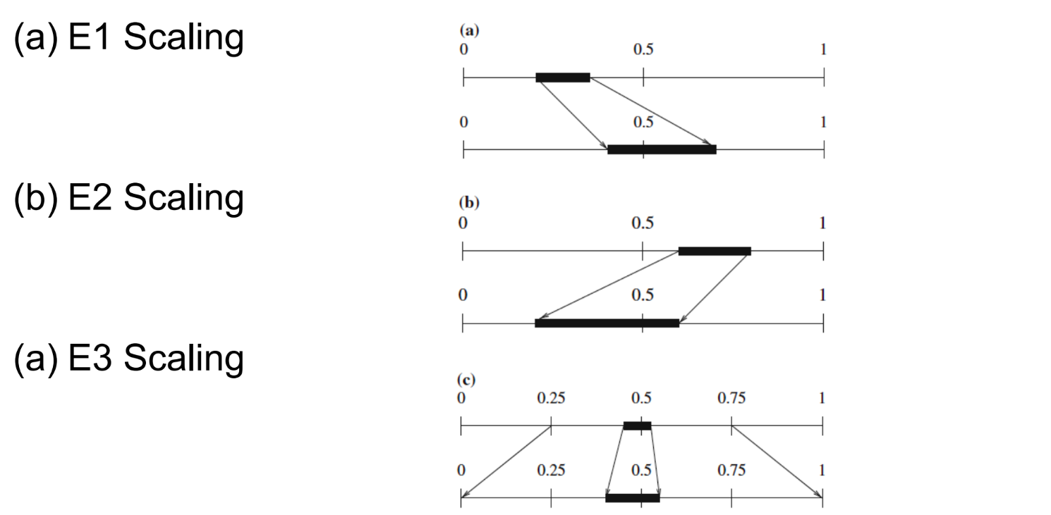
E1:

• send ‘0’ to decoder

• huidig interval volledig in linkerhelft: laagste en hoogste waarde van interval maal 2 (bitshift left)

E2

• send ‘1’ to decoder

• huidig interval volledig in rechterhelft: laagste en hoogste waarde van interval maal 2 en - 0.5 (bitshift left)

E3

• huidig interval tussen 0.25 en 0.75: beide grenzen maal 2 en - 0.25

• signalling iets meer complicated

• One can prove that:

  • N E3 scaling steps followed by E1 is equivalent to E1 followed by N E2 steps

  • N E3 scaling steps followed by E2 is equivalent to E2 followed by N E1 steps

• Therefore, a good way to handle the signaling of the E3 scaling is: postpone until there is an E1 or E2:

  • if there is an E1 after N E3 operations, send ‘0’ followed by N ‘1’s after the E1;

  • if there is an E2 after N E3 operations, send ‘1’ followed by N ‘0’s after the E2.

integer implementation of arithmetic coding

• Uses only integer arithmetic. It is quite common in modern multimedia applications

• Basically, the unit interval is replaced by a range [0, N], where N is an integer, e.g. 255

• Because the integer range could be so small, e.g., [0, 255],applying the scaling techniques similar to what was discussed above, now in integer arithmetic, is a necessity

• The main motivation is to avoid any floating number operations

Binary arithmetic coding (BAC)

• Only use binary symbols, 0 and 1.

• The calculation of new intervals and the decision of which interval to take (first or second) are simpler.

• Fast Binary Arithmetic Coding (Q-coder, MQ-coder) was developed in multimedia standards such as JBIG, JBIG2, and JPEG-2000. The more advanced version, Context-Adaptive Binary Arithmetic Coding (CABAC) is used in H.264 (M-coder) and H.265.

  • symbols are first binarized in a specific (optimized) way (!)

adaptive binary arithmetic coding

• houdt telkens bij hoeveel 0’en of 1’tjes al ontvangen werden en berekend zo de grootte van het interval

• wordt telkens aangepast per ontvangen bit (adaptive)

• voordeel tov adaptive huffman → geen nood aan zeer grote en dynamische symbol table

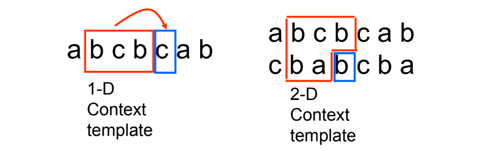
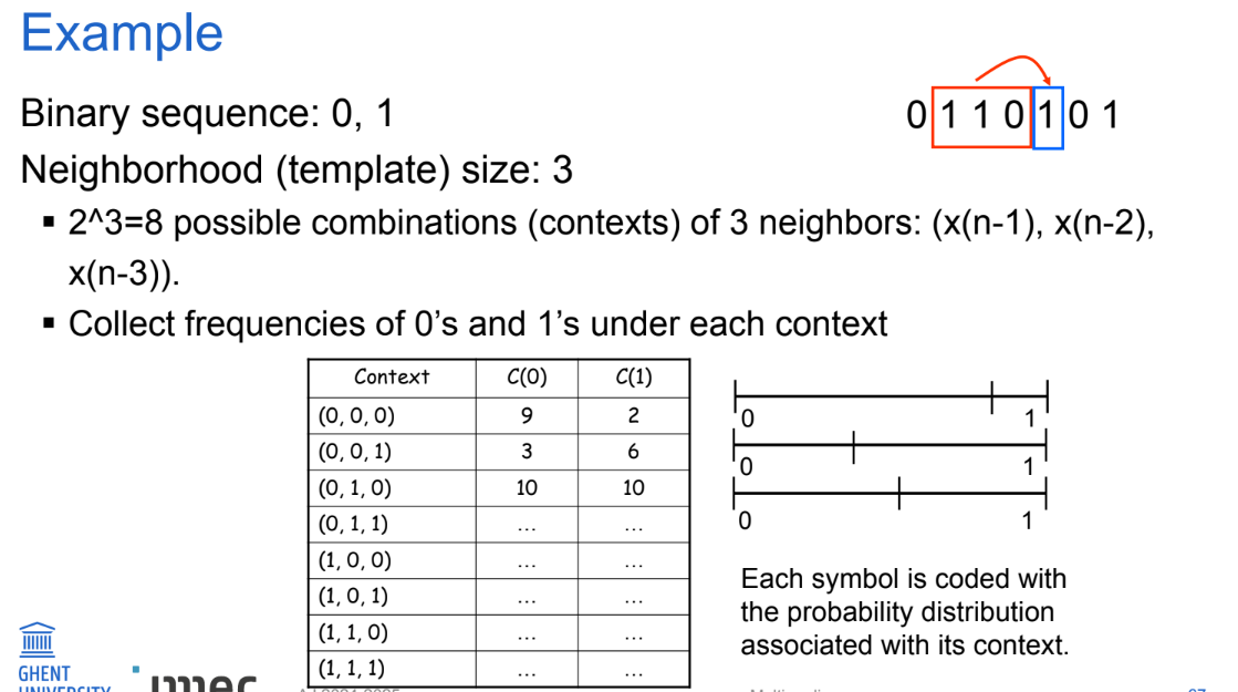
context-adaptive arithmetic coding

• Probabilities → higher-order models

• A sample often has strong correlation with its near neighbors

• Idea:

  • collect conditional probability distribution of a symbol for given neighboring symbols (context): P(x(n) | x(n-1), x(n-2), ... x(n-k))

  • use this conditional probability to encode the next symbol

  • more skewed probability distribution can be obtained (desired by arithmetic coding)

performance arithmetic coding vs huffman coding

For a sequence of length m:

• H(X) <= Average Bit Rate <= H(X) + 2/m

• approaches the entropy very quickly.

Huffman coding:

• H(X) <= Average Bit Rate <= H(X) + 1/m

• Impractical: need to generate codewords for all sequences of length m.

• (cf. Extended Huffman coding)

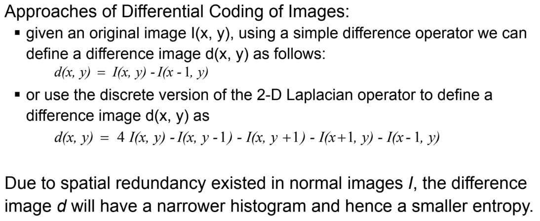
differential coding of images

lossless JPEG

Lossless JPEG: A special case (mode) of the JPEG image compression

Predictive method

• Forming a differential prediction: A predictor combines the values of up to three neighboring pixels as the predicted value for the current pixel, indicated by ‘X’. The predictor can use any one of the seven schemes listed in the table.

• Encoding: The encoder compares the prediction with the actual pixel value at the position ‘X’ and encodes the difference using one of the lossless compression techniques we have discussed, e.g., the Huffman coding scheme.