Probability and Statistics Refresher (Week1)

Quants

Random Variables ?

A variable which takes on a numerical value as a result of a random process

Discrete R.V: The number of outcomes of the random variable are distinct and countable

Continuos R.V: The random variable can take on infinitely many different outcomes

How are Random variables treated in Quant Ecos?

Random variables are treated as continous even though they may technically be discrete

Probability density Functions (PDF’s)

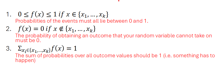
3 properties for a valid PDF:

• f(x) > 0

• The integral of f(x)dx = 1

Bernoulli Random Variable

Special type of discrete random variable with 2 possible outcomes. e.g coin toss

It is descibed by the probability of success (observing 1)

Discrete Random Variable with more than 2 outcomes

If you have more than 2 outcomes, just list the probability that the random variable takes on each of the values

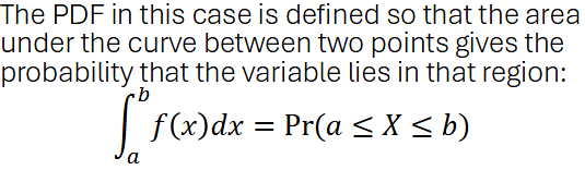
Continuos Random Variables

With CT RV’s, we have infinitely many x-values that our variable can take on. SO the probability of taking on an exact value is 0. Hence, we look at the area between 2 points

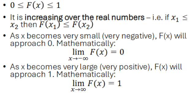
Cumulative Distribution Functions (CDF)

Defined the same for both discrete and continuous rv’s.

F(X) = Pr(X<x) : Which is the probability of observing an outcome as large as x

CDF Properties

Using CDF’s to calculate probabilities

2 properties:

• Pr(x>b) = 1 - F(b)

• Pr (a<X<b) = F(b) - F(a)

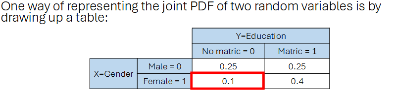
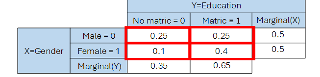
Joint Probabilities

When we have 2 random variables, X & Y, we have a joint distribution

The distribution describes the probability of 2 events happening together.

Joint PDF: f(X,Y) = Pr(X=x,Y=y)

Joint PDF properties

For a joint pdf to be valid:

• joint probabiity values should lie between 0 and 1

• joint probabilites need to sum to 1

Marginal Distributions

A marginal distribution is the probability distribution of a single variable in a multivariable (usually joint) distribution. It is found by summing (for discrete variables) or integrating (for continuous variables) over the other variable(s), effectively "marginalizing out" the others.

Statistical Independence

Two events are statistically independent if:

• Pr(A and B) = Pr (A) x Pr(B)

In the case of 2 random variables, X and Y are statistically independent iff their joint probability is the product of their respective marginal distributions

Proving Statistical indepenence

• To prove statistical independence, we have to show the property holds for all cells.

• To disprove, we need to only show one that fails - then they are statistically dependent

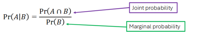
Conditional Distributions

When you want to determine how one of the variables changes if we fix the other one at a specific level.

• Note: If you hold an event fixed, all the distributions containing that event should sum to 1

Conditional distributions and statistical Independence

A conditional distribution will tell you the probability distribution of one random variable, whilst holding the other fixed.

If X and Y are statistically independent, then the cond.distr of x given a value of Y should be the same no matter what we choose to fix Y on.

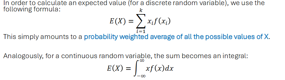
Expected Value operator E(x)

A measure of central tendency. It gives us a measure of the value we expect a random variable to take on. It is also the 1st moment of the distribution.

Note: The expected value of a random variable does not need to be an exact value that the random variable can take on.

Properties of Expected Values E(x)

• If c is a constant, then: E(c)= c

• If a & b are constants, then:

  E(aX+b) = aE(x) + b

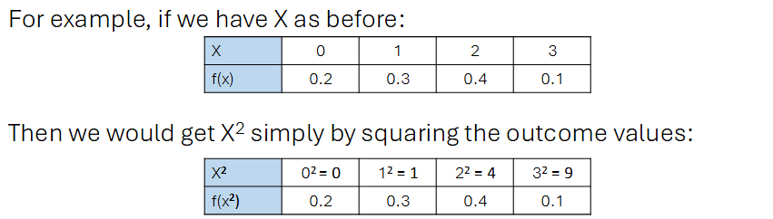
Functions of random variables

Note: If X is a random variable, then X² is also a random variable etc.

• Applying any function to a random variable only changes the outcome with which the random variable can take on, and not the probability distribution of the random variable’s value.

Measures of variability: Variance

Variance - A measure of spread; how far a random variable deviates from its mean. It is also the 2nd moment of the distribution

Var(x) = [E(X-E(X))²] = E(X²) - (E(X))²

Properties of Variance

• Variance of a constant is zero as a constant does not vary at all

• Var(aX + b) = a²var(X)

Standard deviation and its properties

The positive square root of the variance of a random variable. Written as sd(x).

Properties:

• for constant c, sd(c) = 0

• for constants a,b; sd(aX +b) = |a|sd(x)

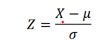
Standardizing a Random Variable

To standardize a variable to obtain a random variable with a distribution with a mean of zero and variance of 1, we subtract by its mean and divide by the standard deviation.

Skewness and Kurtosis

Skewness is the 3rd moment of a distribution. Depicts how skew a random variable is.

Kurtosis is the 4th moment of a distribution. Depcits the thickness of the tails of the distribution.

Relationship between covariance & correlation

Linked in the sense that the correlation between 2 variables is simply the covariance adjusted for the standard deviations of those variables.

Both concepts refer to the notion of how 2 variables move together

What is covariance

The covariance between 2 random variables measures the amount of linear dependence between 2 random variables. Written as, Cov(X, Y)

Note:

• +’ve Cov: X and Y move in the same direction

• -’ve Cov: X and Y move in opposite directions

Cov(X,Y) = E(XY) - E(X)E(Y)

Cov(X,X) = Var(X)

Properties of Covariance

• If X & Y are independent, then Cov(X,Y) = 0, however the reverse is not always true

• Cov(a1X+b1, a2Y+b2) = a1a2Cov(X,Y)

• |Cov(X,Y)| < sd(X)sd(Y)

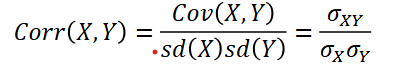
The Correlation Coefficient

Corr(X,Y) is the covariance betwen X and Y standardized by their standard deviations.

Properties of Correlation

• -1 < Corr(X,Y) < 1

• if a1,a2 > 0, then Corr(a1X+b1,a2Y+b2) = Corr(X,Y)

• if a1,a2 <0, then Corr(a1X+b1,a2X+b2) = -Corr(X,Y)

  Reflects that the Correaltion coefficient is scale independent

Variances of sums of Random Variables

What if you want to calculate the variance of a newly created random variable due to a sum of 2 random variables?

Var(aX + bY) = a²Var(X) + b²Var(Y) + 2abCov(X,Y)

• If x and y are uncorrelated, then the covariance term drops

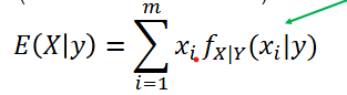
Conditional Expectation

The conditional expectation operator is one that calculates the expected value of one random variable, while holding the other fixed at some particular value.

Properties of condtional expectations

• E[c(x) | X] = c(X); functions of X are treated as constants when we control for X

• If X and Y are independent, then E(Y|X) = E(Y), then Cov(X,Y) = 0

• For functions a(X) and b(X), E[a(X)Y + b(X)|X] = a(X)E(Y|X) + b(X)

• Ex[E(Y|X)] = E(Y)

Conditional Variance

Var(Y|X=x) = E(Y²|x) - [E(Y|x)]²

• If x and y are independent, then Var(Y|X) = Var(Y)

The normal distribution

Characteristics of a normal distribution:

• skewness = 0 and kurtosis = 3

• STD normal will have a mean of 0 and varinace of 1

• X~Normal(mew, sigma²)

The standard normal table

Calculating probabilities using tables:

• Have to standardize your random variable first

• Area under a std normal curve is 1

• The table gives the area under the curve to the left of your particular number

Estimates and Estimators

An estimator of a parameter theta is a rule that assigns each possible sample a value of theta.

Once you apply the rule to a particular data, you obtain an estimate.

Unbiasedness

How well does an estimator estimate the true parameter value?

We can check by determining whether an estimator is unbiased or not:

• An estimator, W, of a parameter theta is unbiased if E(W) = theta

• If it ‘s biased, then E(W) = theta + Bias(W)

  Note: Bias(W) = E(W) - theta

Sampling Variances

Unbiasedness alone is not good enough to conclude whether an estimator is good or not;

Thus another metric of how precise an estimator predicts the populaton parameter is the sample variance of the estimator.

• What is the spread of values the estimator gives us.

Efficiency of an Estimator

We want to determine which of our estimators are more useful than others. Naturally we want our estimators to be unbiased and precise as possible. Hence, ideally the lower the sampling variance, the better.

Efficiency:

• If Var(W1) < Var(W2), the W1 estimator is more efficient

Consistency

What happens to your sampling distribution of your estimator as you increase the size of the sample you draw from the population.

An estimator is consistent if:

• It is unbiased

• The sampling variance goes to zero as the sample size (n) increases.