MTH 267 - Differential Equations Exam 1 Topics

Module 1: Introduction to Differential Equations, Module 2: First-Order Differential Equations, Module 3: Modeling with First-Order Differential Equations

Ordinary Differential Equation (ODE)

ordinary derivatives w.r.t. 1 Independent Variable (IV)

Partial Differential Equation (PDE)

partial derivatives w.r.t. 2 or more IVs

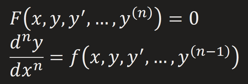
Normal Form ODE

F: real-value function of n+2

y^(n): highest derivatives in terms of n+1

f:real-valued continuous function

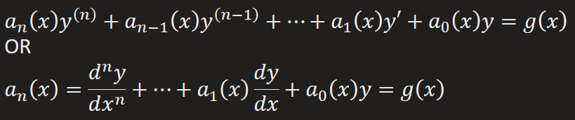
Linear

Steps:

1) Convert given equation to the general linear formula by…

(a) dividing all terms by dx when x = IV

(b) collecting y terms (DV) on the left & x terms (IV) on the right

2) Compare to general linearity formula to verify it matches

Solution

“any function, defined on an interval I, with n continuous derivatives that satisfies the equation identically when substituted into it”

Interval (I)

interval of definition, interval on which a particular solution to the ODE is defined

Verification of Solution

substitute & determine whether each side of the equation is the same for every x in I

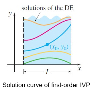
Solution Curve

graph of a solution to an ODE 

1) They do NOT cross equilibrium lines & can NOT change signs

2) They either always go up or always go down (monotonic) - above or below

3) They eventually settle near equilibrium pts. - Bounded (between c₁ & c₂)

Implicit Solution

“G(x,y)=0 of an ODE on I given that there exists 1 function that G(x, y(x))=0,” relating x & y w/o explicitly solving for y

Trick: rewrite y as y(x) to indicate that dy/dx will be needed

Families of Solutions

set of relation functions with arbitrary Constant (C)

Singular Solution

solution that’s NOT a member of the family of solution

nth-Order Initial Value Problem (IVP)

“on some interval I containing x₀ the problem of solving an nth order differential equation subject to n side conditions specified at x₀”

Steps:

1) Plug in 1st Initial Condition (IC)

2) Plug in 1st parameter

3) Differentiate

4) Plug in 2nd IC
5) Plug in 2nd parameter

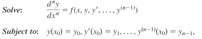
First-Order IVP

n=1

Solve: dy/dx=f(x,y)

Subject to: y(x₀)=y₀

Point (pt.)

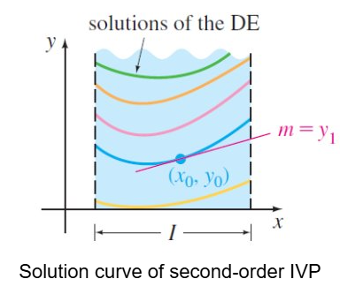
2nd-Order IVP

n=2

Solve: d²y/dx²=f(x,y,y’)

Subject to: y(x₀)=y₀,y’(x₀)=y₁

Slope

Existence & Uniqueness

“Let R be a rectangular region in the xy-plane defined by a ≤ x ≤ b, c ≤ y ≤ d that contains pt. (x₀,y₀). If f(x,y) & ∂f/∂y are continuous on R, then there exists some I₀: (x₀ - h, x₀ + h), h ≥ 0, contained [a, b] & a unique function y(x)”

Note: I of definition does not have to be as wide as R & the I₀ of existence & uniqueness might not be as large as I

Steps:

1) Continuous f(x,y) gives existences, so identify f(x,y)

2) Continuous ∂f/∂y gives uniqueness, so compute ∂f/∂y

3) Find where f(x,y) & ∂f/∂y are continuous

(a) No divisions by 0

(b) No even roots of negative numbers

(c) No logarithms of zero or negative numbers.

(d) No undefined expressions like 0/0 or ∞/∞

(e) No discontinuities in trigonometric functions (e.g., avoid tan(x) at x=2π+kπx ).

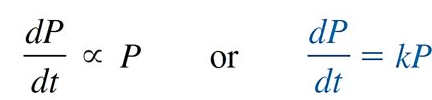
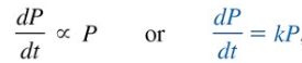
Population Growth

“rate of population growth at a time is proportional to the population at that time”

P(t) = population at time (t)

k = constant of probability

P(t) = P₀(t)e^kt

Note: It is decay if k < 0.

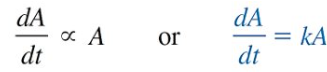
Radioactive Decay

“the rate dA/dt at which the nuclei of a substance decay is proportional to the amount A(t) of the substance remaining at time t”

A(t) = A₀e^-kt

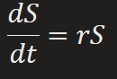
Compound Growth

“growth of capital S when annual rate of interest r is compounded”

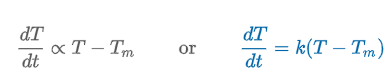
Newton’s Empirical Law of Cooling/Warming

“the rate at which temperature (temp.) of a body changes is proportional to the difference between temp. of body & ambient temp.”

T(t) = T_m + (T₀ -T_m)e^kt

T(t) = temp. of body at time t

T_m = ambient temp.

k = constant of probability

k > 0: warming

k < 0: cooling

Spread of Disease

“the rate dx/dt in which the disease spread is proportional to the number (#) of interactions between diseased people x(t) & unexposed people y(t)”

1^st Order Chemical Reactions

“disintegration of a radioactive substance”

X(t) = amount of substance A at any time t

k = negative constant

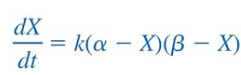
2^nd Order Chemical Reactions

“disintegration of a radioactive substance”

X(t) = amount of C at time t

α = amount of A

β = amount of B

α - X = amount of A not converted to C
β - X = amount of B not converted to C

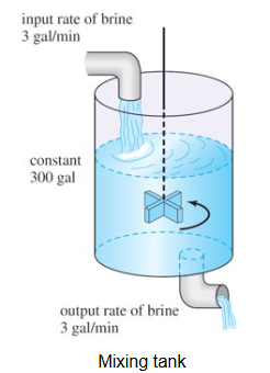
Mixture

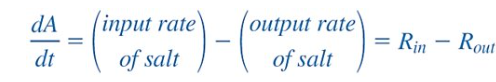
“the amount of salt in a mixture of 2 salt solutions of differing concentrations”

A(t) = amount of salt in tank at time t

R_in = input rate of salt

R_out = output rate of salt

R = concentration * rate

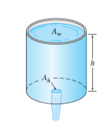
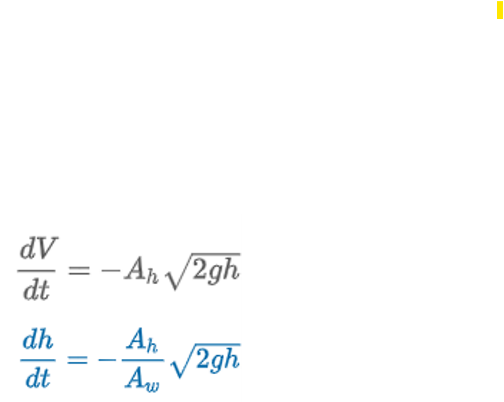
Draining a Tank

“Torricelli’s Law states that the speed of which a fluid flows out of a hole of a container is equal to the speed of it falling freely from the height of the fluid’s surface to the level of the hole.”

A_h = area (ft³) of hole

v = √2gh = speed (ft/s) of water leaving the tank

V(t) = A_wh = volume of water leaving the tank at time t

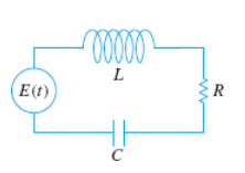
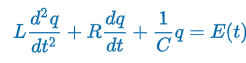
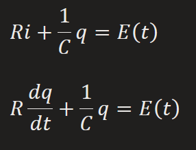
LRC Series Circuit

“Kirchoff’s 2^nd Law states the impressed voltage E(t) in a closed loop equals the sum of the voltage drop.”

E(t) = impressed voltage

i(t) = current in closed circuit

q(t) = charge incapacitor at time t

L = inductance

R = Resistance

C = Capacitance

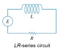
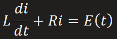
LR Series Circuit

E(t) = impressed voltage

i(t) = current in closed circuit

q(t) = charge incapacitor at time t

L = inductance

R = Resistance

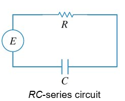
RC Series Circuit

E(t) = impressed voltage

i(t) = dq/dt current in closed circuit

R = Resistance

C = Capacitance

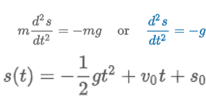
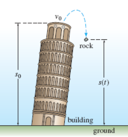
Falling Bodies

“Newton’s 1^st law states a body in motion remains in motion & a body at rest remains at rest unless acted upon by a force. Newton’s 2^nd Law states Force = mass * acceleration.”

s(t) = height position of falling object (obj.)

d²s/dt² = acceleration of falling obj.

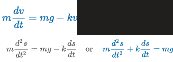
Falling Bodies w/ Air Resistance

“when air is proportional to velocity”

mg = F₁ = W

-kv = F₂ = viscous damping

W = weight

m = mass

g = gravity

s(t) = distance body falls

ds/dt = v = velocity

d²s/dt² = dv/dt = a = acceleration

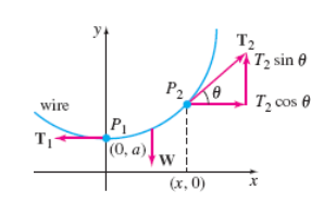
Suspended Cables

“3 forces act on the cables - tension T₁ (tangent to P₁), tension T₂ (tangent to P₂), & Weight W (between P₁ & P₂)

T₁ = cosθ

W = T₂sinθ

tanθ = W/T₁

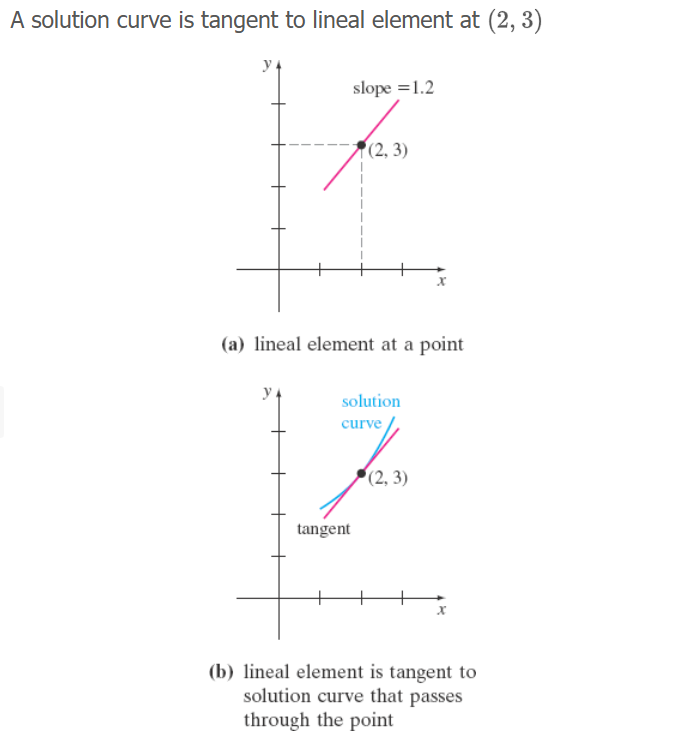
Lineal Element

“the value f(x,y) that the function f assigns to the pt. represents the slope of the line segment,” dy/dx = m

Note: passing through pts. on any horizontal line must have the same slope & is parallel; slope of lineal along any vertical line vary

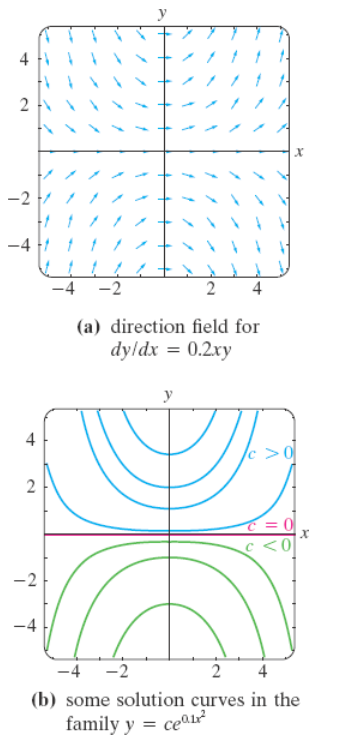
Direction Field / Slope Field

“collection of all line elements at each pt. (x, y) of a rectangular grid w/ slope f(x,y); appearance/shape of a family of solution curves of the differential equation”

“A single solution curve that passes through a direction field must follow the flow pattern of the field; it is tangent to a lineal element when it intersects a point in the grid”

Note: both definitions are true, recall whichever phrasing is the most helpful for you

Autonomous

an ODE in which the IV does not appear explicitly

Phase Line Example

P(a - bP) = 0 → P = 0, a/b

Interval | Sign of f(P) | P(t) | Arrow

(-∞, 0) | minus | decreasing | down

(0, a/b) | plus | increasing | up

(a/b, ∞) | minus | decreasing | down

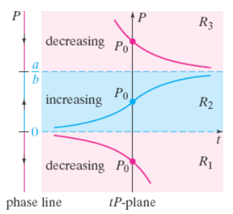
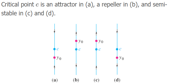
Asymptotically stable/Attractor, Unstable/Repeller, Semi-Stable

Asymptotically stable/Attractor: when the arrowhead of both sides point towards c; lim x→∞ y(x) = c

Unstable/Repeller: when the arrowheads of both side point away c

Semi-Stable: both attracts & repels

Translation Property (of an autonomous DE)

“If y(x) is a solution of an autonomous DE dy/dx = f(y), then y(x) =y(x -k), k = constant, is also a solution.”

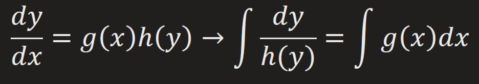
Separable 1^st Order DE

can be separated as a product of a function of x & a function of y (can be linear or nonlinear)

Steps:

1) Separate y terms on the right & x terms on the left

2) Integrate

3) If asked, solve for y

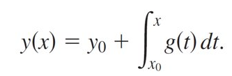
Integral Defined Function

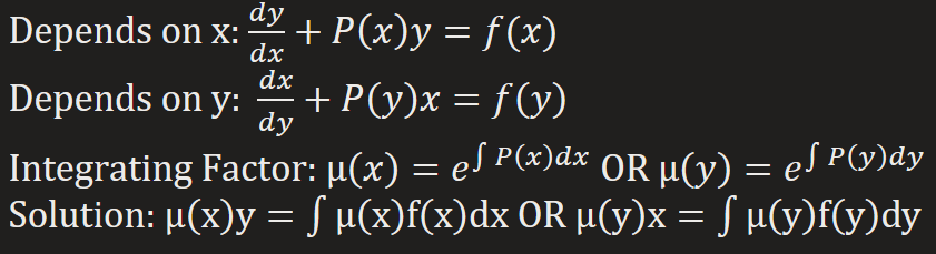
Linear 1^st Order DE

Follows the linear general formula: a₁(x)(dy/dx) + a₀(x)y = g(x)

Steps:

1) Put into standard form; (dy/dx) + P(x)y = f(x)

2) Identify P(x) & find the integrating factor: μ = e^∫P(x)dx

3) Multiply both sides of the standard form by the integrating factor. The LHS of the resulting equation is the derivative of the product of integrating factor & y.

4) Integrate both sides of the last equation.

5) If asked, solve for y

Transient Terms

We say that ce^-x is a transient term, since e^-x → 0 as x → ∞

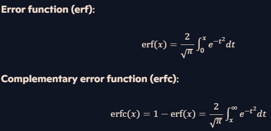
Error Function

defined in terms of nonelementary integrals

Exact 1^st Order DE

Differential is continuous & has continuous 1^st partial derivatives in R defined by a < x < b & c < y < d on some function f(x,y)

Steps:

1) Set in Exact Equation

2) Integrate w.r.t. x / Integrate w.r.t. y

3) Partial Differentiate w.r.t. y / Partial Differentiate w.r.t. x

4) Integrate h’(y) / Integrate g’(x)

5) Final answer = C

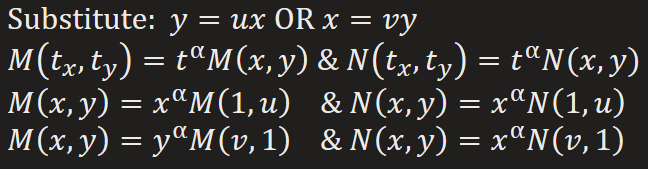
Homogenous 1^st Order DE

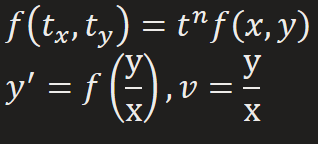
Homogenous & Exact 1^st Order DE

The Exact equation, M(x,y)dx + N(x,y) = 0, is Homogenous if the coefficient functions M(x,y) & N(x,y) are homogenous functions of the same degree (where α is equal to one another)

Substitute y = ux or x = vy

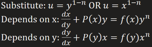
Bernoulli 1^st Order DE

Can be reduced to a linear equation by means of substitution (linear & separable)

How do you determine which 1^st - Order DE strategy to implement?

1) Separability → Separable

2) Linearity → Linear

3) Exactness (w/ or w/o Integrating Factor) → Exact

4) Single Nonlinearity → Bernoulli

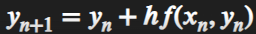
Euler’s Method

Linearization of the unknown solution of y’(x) = f(x, y) , y(x₀) = y₀

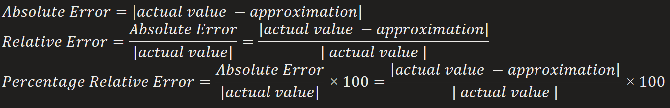
Absolute Error, Relative Error, Percentage Relative Error

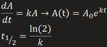
Half-Life

“time it takes for ½ of the atoms in an initial amount A₀ of a radioactive substance to transmute into the atoms of another element,” measuring the stability of a radioactive substance

Carbon Dating

“comparing the proportionate amount of C-14 in a fossil w/ constant ratio found in the atmosphere to estimate an age”