Statistics 2 Lecture 4

Effect sizes in multiple regression

• Typically, we are also interested in the explanatory power of single predictors in the model.

• For multiple regression holds: We cannot use b to judge the strength of the partial association between x and y

• → b depends on the scale on which x and y were measured.

• Solution: Inspect the effect size

• For multiple regression we have various options:

  • Standardized regression coefficient: b*

  • Squared partial correlation: 𝑟p2

  • Change in explained variation: Δ𝑅2

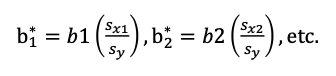
Standardized regression coefficients (b*)

• We can scale each of the b coefficients in the multiple regression model using the:

  • SD of the respective predictor (x)

  • SD of the outcome variable (y)

• Interpretation: The amount of SDs y is expected to change when x increases with 1 SD (controlling for all other predictors in the model)

• Rules of thumb for interpretation

  0 < negligible < .10 ≤ small < .30 ≤ moderate < .50 ≤ large

• Thus works the same as in simple regression but:

  • Not simply Pearson’s correlation (r) between x and y

  • That’s because we statistically control for the other predictors in the model

(Squared) Partial correlation

• The (squared) partial correlation is defined in terms of the correlations instead of the b coefficient itself.

• Example:
  In a model with two predictors (x1 and x2).
  The partial correlation between x1 and y, Controlling for x2

• proportion variation in y uniquely explained by x1 / proportion variation in y not explained by x2

• Rules of thumb to interpret 𝑟2: 𝑝

  0 < negligible < . 01 ≤ small < .06 ≤ moderate < .14 ≤ large

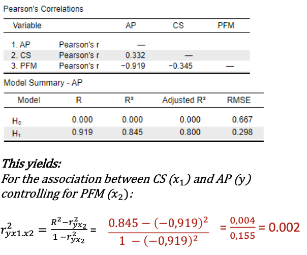
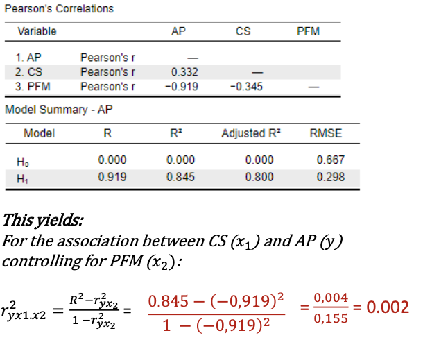
Squared partial correlation example

Class size explains 0.2% of the differences in academic performance that were not yet explained by the percentage students with free meals.This is a negligible effect.

R-squared change

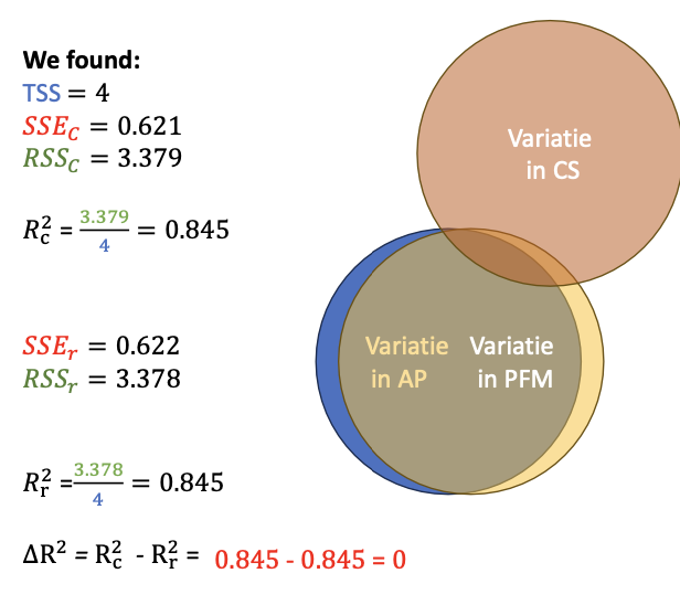
• Effect size ΔR2 is defined as the difference in explained variation when we compare two models.:

• A complete model: With all predictors

  • Example: y = a + b1×1 + b2×2

• A Reduced model: Including all predictors, apart from the one for which you want to know the partial effect

  • Example: y = a + b1×1

• R-squared change: ΔR = Rc - Rr

• Interpretation: The proportion variation in y uniquely explained by x2.

• Rules of thumb for interpretation

• 0 < negligible < .02 ≤ small < .13 ≤ moderate < .26 ≤ large

R-squared change example

Class size explains 0% of the differences in academic performance, above and beyond the differences that were already explained by differences in the percentage of students with free meals.

Familiar rules applied to model c and model r

• Rule 1: When we predict 𝑦 with x1: → The prediction equation 𝒚ෞ = 𝒂 + 𝒃𝒙 makes the best prediction.

• Rule 2: When we predict 𝑦 with x1 and x2: →The prediction equation 𝒚ෞ = 𝒂 + 𝒃 𝒙 + 𝒃 𝒙 makes the best prediction.

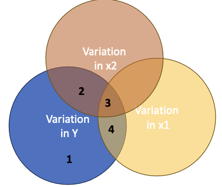
• Prediction errors: Is the difference between the observed and the predicted y of a subject:Variation in x2

• →With rule 1: error = 𝑦 − 𝑦ෝ 𝑟2 summarized (over subjects) as 𝑆𝑆𝐸r = ∑ (𝑦 − 𝑦r)2 = SSE in the reduced (H0) model

  • In the Venn-diagram: 𝑺𝑺𝑬𝒓 = 1 + 2

• Va→With rule 2: error = 𝑦 − 𝑦ෝ summarized (over subjects) as 𝑆𝑆𝐸c ∑ (𝑦 − 𝑦c)2 = SSE in the complete (HA) model

  • In the Venn-diagram: 𝑺𝑺𝑬𝒄 = 1

• Question we could ask: Does the complete model perform significantly better in predicting y than the reduced model

The F-test for model comparison

• Variation uniquely explained by additional parameters complete model / df1

• Variation that remains unexplained / df2

• By comparing a complete model and a reduced model that differ by one b coefficient

• We test: H0: 𝛽𝑖 = 0

• Compares the residual sums of squares (SSE) of:

  • Complete model

  • Reduced model

• Test the explanatory power of the extra predictors in the complete model.

• Models can be extended with more parameters as long as the reduced model is a simplified version of the complete model. →The models should be nested.

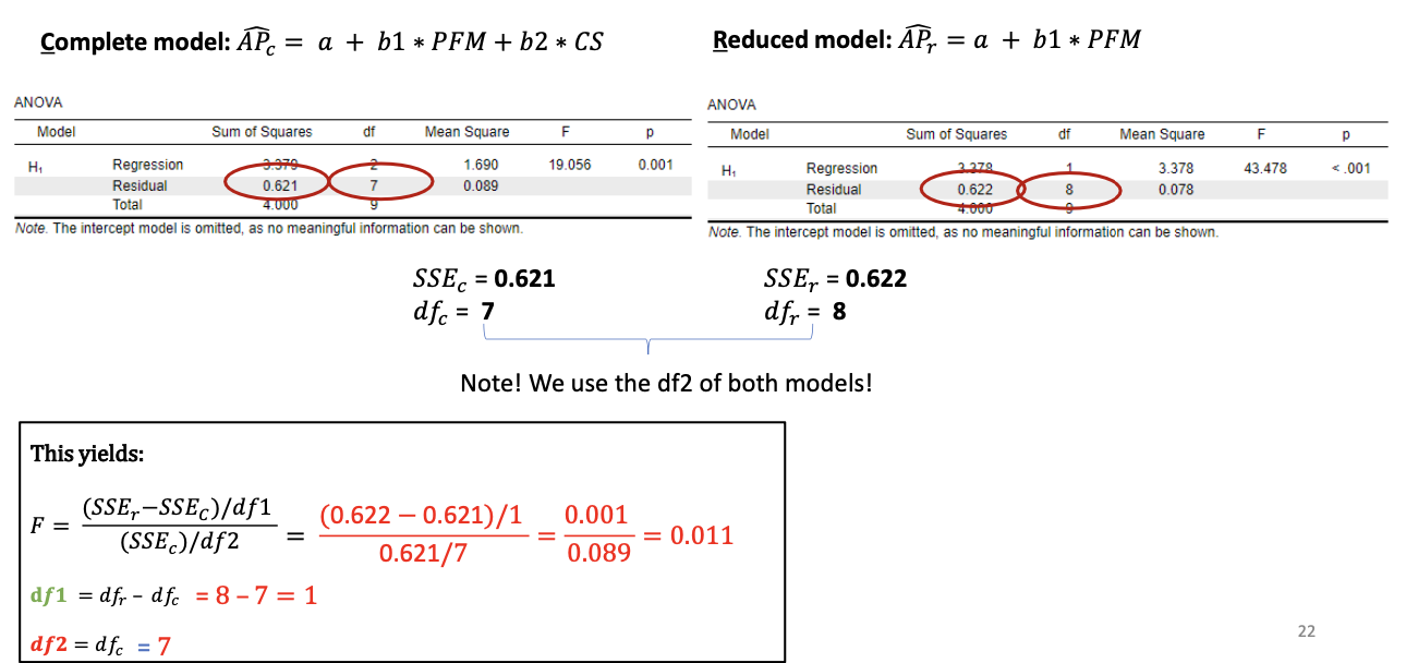
• Our example:

• Complete model: 𝑦ො = 𝑎 + 𝑏1𝑥1 + 𝑏2𝑥2 = a + b1*PFM + b2*CS →Reflects the HA that the partial effect of CS, b2 ≠ 0

• Reducedmodel:𝑦ො= 𝑎 + 𝑏1𝑥1 =a+b1*PFM
  →Reflects the H0 that the partial effect of CS, b2 = 0

• F-test significant? Reject H0, Conclude that the additional parameter is significant: here, b2 ≠ 0.

• F-test not significant? No evidence to reject the H0