Honours Differential Equations

How do we change an nth order ODE into first order?

1. change variables to x1 = y, x2 = y’ etc… xn = y^(n-1)

2. Take derivatives of new variables

autonomous definition

If F is a function of only x, ie δ_tF = 0

Abels Thm

If W(t₀) ≠ 0 for some t₀ then W(t) ≠ 0 for all t

How to solve homogenous system with constant coefficients?

1. Find eigenvalues and eigenvectors of A

2. if real and different eigenvalues then x = sum(c_ne^r_nξ_n)

3. If complex eigenvalues then x = c₁u(t) + c₂v(t) + ….. where u(t) = e^rt(acos(μt) - bsin(μt)) and v(t0 = ie^rt(bcos(μt) + asin(μt))

4. If repeated eigenvalues then x(t) = c₁e^rt ξ + c₂(te^rt ξ + e^rtη)

   1. can extend by just adding extra unknown vectors, e.g. if 3×3 then our 3rd solution is (t²/2)e^rt ξ + te^rtη + e^rtζ

Fundamental Matrix

ψ(t) = nxn matrix with fundamental solutions as columns

det(ψ(t)) = 0

x(t) = ψ(t)c

Matrix Exponentials

e^At = I + At + (1/2!)A²t + …

e^A+B = e^Ae^B if AB = BA

e^0t = I

e^At = ψ(t) for ψ(0) = I

x(t) = e^Atx(0) <=> e^At = ψ(t)ψ^-1(0)

if T is diagonalisable then e^At = Tdiag (e^r₁t , e^r₂t , . . . , e^r_nt )T ⁻¹

Variation of Parameters for non homogenous ODEs

1. dx/dt = P(t)x + g(t)

2. assume the homogenous part is solved by x_hom = ψ(t)c

3. introduce x = Ψ(t)u(t) which we differentiate and sub into 1 to get Ψ (t)u(t) + Ψ(t)u (t) = P(t)Ψ(t)u(t) + g(t)

4. This reduces to Ψ(t)u (t) = g(t) since Ψ′ = P(t)Ψ

5. Thus u(t) = integral (Ψ⁻¹(t)g(t))dt + u(t₀)

6. so x(t) = Ψ(t)Ψ⁻¹(t₀)x₀ + Ψ(t) * integral(t₀-t)Ψ⁻¹(s)g(s) ds
   

Diagonalisation for non homogenous ODEs

1. assume the corresponding homogenous system is solved with r_i and ξ_i 

2. We introduce a change of variables x = Ty so Ty = ATy + g(t) => y = (T−1 AT)y + T−1 g(t) = Dy + h(t)

   1. note that T is normalised

3. We now have a system of n decoupled equations which we can solve by direct integration

4. If not diagonalisable then can use jordan form instead but note that won’t be decoupled so have to solve in correct order

Undetermined Coefficients for non homogenous ODEs

guess a solution for the non homogenous part and add to homogenous solution

need ate^λt + be^λt if g = ue^λt

Stable critical point definition

if for all ε there exists δ > 0 such that every x(t) with |x(0)-x₀| < δ satisfies lim (x(t)) = x₀

asymptotically stable if its stable and attracting

Attractive critical point definition

if there exists δ > 0 such that every x(t) with |x(0)-x₀| < δ satisfies lim (x(t)) = x₀

ie if we start close the the critical point then we tends to it

Almost Linear systems

If we have x’ = F and y’ = G then we approximate this linearly by saying u’ = Au and u = x - x₀ where A = a matrix with rows F and G and differentiating in columns by x and y

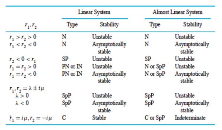
Critical points table for linear and almost linear systems

If table is not helpful then we can explicitly solve (may be helpful to switch to polar) or try plotting implicit trajectories

Conservation of Energy

dE/dt = (∂_x E )x + (∂_y E )y= ∇E · T (x, y ) = |∇E ||T | cos φ = 0 from conservation of energy

Thus the gradient vector and tangent vector are orthogonal

(semi)definite

Let E : D ⊂ R² → R be defined on a domain D containing a
critical point x0.
E is positive [negative] definite if E (x₀) = 0 and
E (x, y ) >(<) 0 ∀ (x, y ) != x₀
E is positive [negative] semi-definite if E (x0) = 0 and
E (x, y ) ≥(≤) 0 ∀ (x, y )

Lyapunov’s 1st theory

Consider a two-dimensional autonomous system with an isolated critical point x₀ and a region D ⊂ R² containing x₀. Suppose that there is a positive definite and continuous function E : D → R with continuous first partial derivatives, such that E (x0) = 0. If ∂_xEF + ∂y EG is negative semi-definite [negative definite] on D [on D \ {x0}] then x0 is a stable critical point [asymptotically stable critical point ]

E is not necessarily energy here, have to guess E

Lyapunov’s 2nd theory

Suppose that there is a continuous function E : D → R with continuous first partial derivatives, such that E (x₀) = 0 and that in every neighbourhood of (x₀) ∃ at least one point x1 where E (x1) > 0. If ∂_x E F + ∂_y E G is positive definite on D then x0 is an unstable critical point

limit cycle

Limit cycles are closed trajectories such that at least one other
non-closed trajectory asymptotes to them as t → ∞ or t → −∞

Existence of Limit Cycles

given x’ = F (x, y ) , y’ = G (x, y )

1. Let F (x, y ), G (x, y ) have continuous first partial derivatives in
   some simply connected domain D. Then a closed trajectory in D
   must necessarily enclose at least one critical point. If it encloses
   only one critical point, it can not be a saddle point.
   Bernd Schroers Honours Differential Equations

   1. 
      if a simply connected D contains no critical points ⇒ no closed trajectories in D,

   2. if a simply connected D contains a unique critical point and it is a saddle ⇒ no closed trajectories in D

2. Let F (x, y ), G (x, y ) have continuous first partial derivatives in a simply connected domain D. If the divergence ∂x F + ∂y G has the same sign in D then there are no closed trajectories in D

Poincare-Bendixson theorem

Let F (x, y ), G (x, y ) have continuous first partial derivatives in a
two-dimensional domain D. Let D1 be a bounded subdomain of D
and let R consist of D1 and its boundary. Suppose R has no critical points. If ∃ a solution (x(t), y (t)) staying in R ∀ t ≥ t0 then either the solution has a closed trajectory or it spirals towards one. Either way, ∃ a closed trajectory

Fourier Convergence Theorem

The series converges to f (x) ∀ x where f (x) is continuous and to
[f (x+) + f (x−)]/2 at all points where f (x) is discontinuous

even and odd functions

A function f (x) is even if f (−x) = f (x).
A function f (x) is odd if f (−x) = −f (x)

Even: integral between L and -L = 2*integral between 0 and L

Odd: integral between L and -L = 0

Even: Only have cos in foureir

Odd: Only have sin

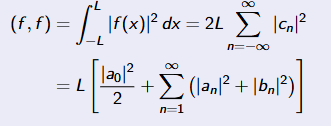
Parsevals Identity

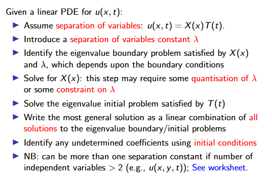
Separation of Variables method

method for non homogenous boundary conditions

1. define v (x) = lim u(x, t)

2. map to one with homogenous boundary conditions

3. u(x, t) = v (x) + ω(x, t)

What is Laplace’s equation in polar coords?

δ²u/δr² + (1/r2)δ²u/δθ² + (1/r)δu/δr = 0

Sturm-Liouville form

− [p(x)y′(x)]′ + q(x)y(x) = λr(x)y(x)

Sturm-Liouville boundary conditions

a₁y(0) + a₂y′(0) = 0

b₁y(1) + b₂y′(1) = 0

Lagrange’s identity

(L[u], v) = (u, L[v])

inner product

(u,v) = integral(0,1)[u(x)v*(x)]dx

⟨Ψ₁, Ψ₂⟩ = integral(0,1)[rΨ₁Ψ₂]dx = 0 if 1 ≠ 2

S-L properties

real eigenvalues

orthogonal eigenvectors

often useful to work with orthonormal eigenfunctions

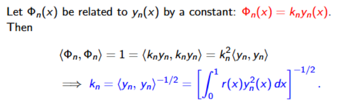
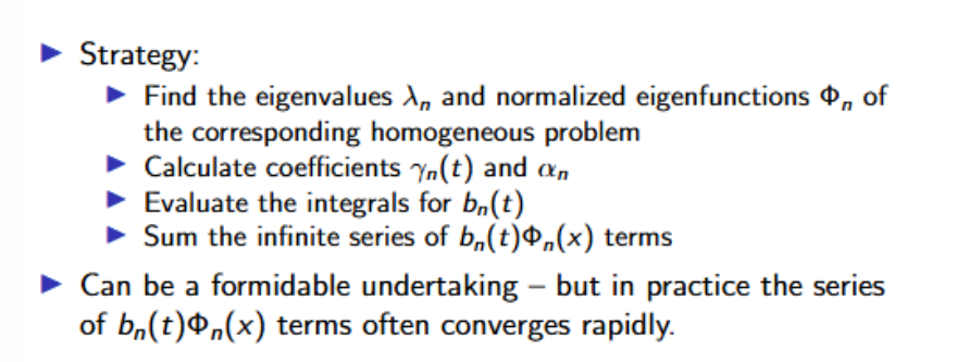
S-L solution

f(x) = sum(c_nΦ_n(x))

where c_n = integral(0,1)[rfΦ_n]dx

self-adjoint problems

needs to be of even order so (L[u],v) = (u,L[v])

non-homogeneous S-L ODEs

1. solve corresponding homogeneous

2. expand to non homogenous

   1. y(x) = sum(b_nΦ_n(x))

3. sub into ODE

   1. sum(b_n(λ_n − μ)Φ_n(x) = f/r

4. expand rhs 

   1. f/r = sum(c_nΦ_n(x)) with c_n = integral(0,1)[Φ_n(x)r(x)f(x)/r(x)]dx

5. so we have sum((b_n(λ_n − μ)-c_n)Φ_n(x)) = 0 thus each coefficient must disappear 

solution: if μ ≠ λ_n then b_n = c_n/(λ_n − μ)

else we either have c_m = 0 so no unique solution

or no solution as all

non-homogenous PDEs

singular S-L

test if Lagranges identity still holds

so need integral(0,1){L[u]v - uL[v]}dx = 0

if 0 singular replace 0 with ε and use limits

need limϵ→0 p(ϵ) [u′(ϵ)v (ϵ) − u(ϵ)v ′(ϵ)] = 0

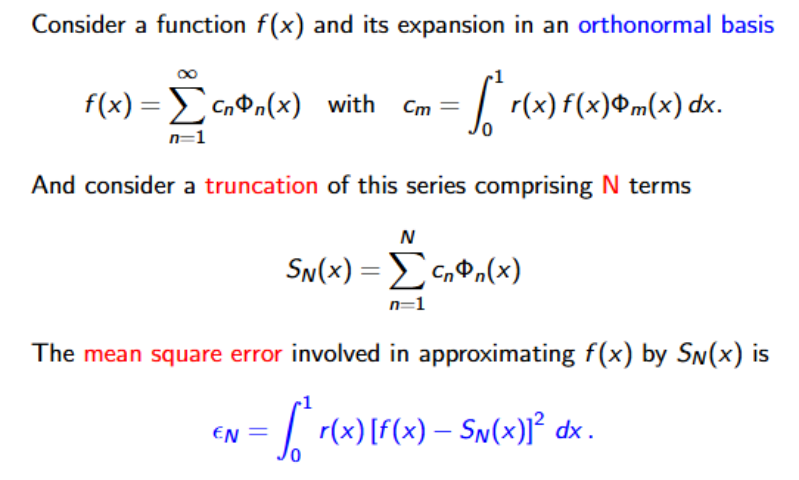
S-L and convergence

if ε_N goes to 0 then the series converges in the mean to f(x)

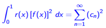
Parsevals identity for S-L

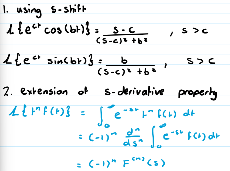
Laplace transform properties

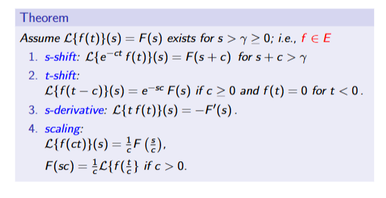
Laplace transform generalisations

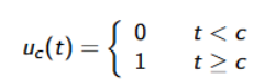
unit step function

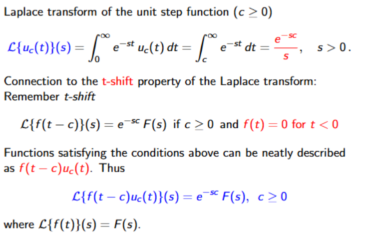
Laplace transform of unit step function

Laplace for non-homogenous ODEs

1. compute L{y} = Y(s) and L{f} = F(s)

2. use partial fraction decomposition

3. find inverse laplace transform using t-shift

   1. L{f(t-c)u_c(t)}(s) = e^-scF(s)

Impulse

take integral(g) = I(τ) = 1 and lim(τ→0)dτ(t) = 0 for t≠0 where g(t) = dτ(t) = some function if -τ<t<τ and 0 otherwise

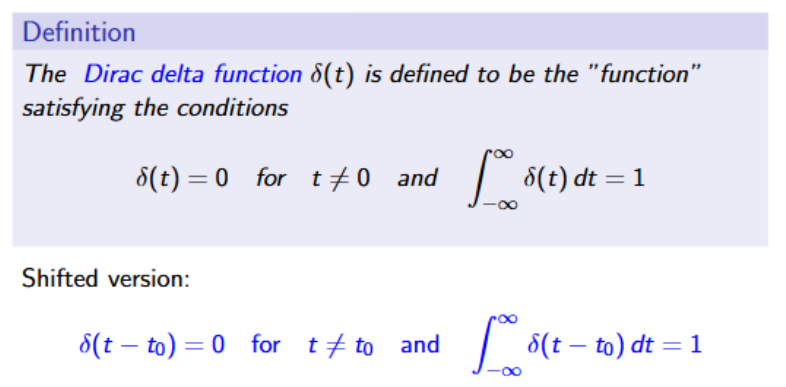
Dirac Delta function

If nice f(t) then the integral(δ(t-t₀)f(t)dt = f(t₀)

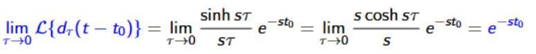
Laplace transform of dirac delta function

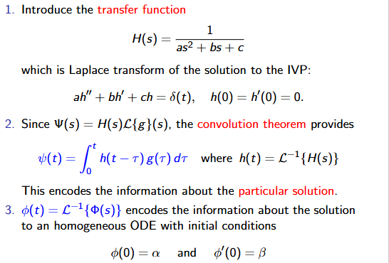
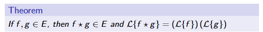
Convolution Theorem

Can use to compute inverse laplace by viewing P = FG

Convolution for non-homogeneous ODEs

Ca use for integral equations