Lvl2: Quantitative Methods

Dependent variable is continuous vs discrete

Continuous: the traditional regression model

Discrete: logistic regression

Regression Process

1. Analyze the residuals

2. Examine the goodness of fit - significance of fit

Assumptions in a simple regression

1. Linearity - Dependent & independent

2. Homoskedasticity - same variance of regression residuals

3. Independence of errors - observations are independent; regression residuals are uncorrelated

4. Normality - regression residuals normal distribution

5. Independence of independent variables - not random; no linear relation between ind variables

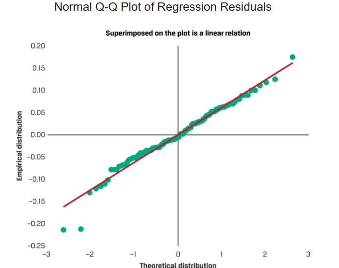
normal Q-Q plot

visualize the distribution of a variable (regression residual) by comparing it to a normal distribution

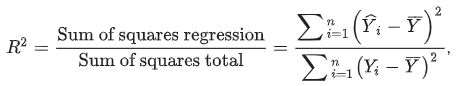
coefficient of determination (R-squared)

ratio of the variation of the dependent variable explained by the independent variables (sum of squares regression) to the total variation of the dependent variable (sum of squares total)

Disadvantages of R-squared

1. cannot provide information on whether the coefficients are statistically significant

2. biases in the estimated coefficients and predictions

3. cannot tell whether the model fit is good - bad model may have a high R² due to overfitting and biases in the model

overfitting

model is too complex - too many independent variables relative to the number of observations in the sample

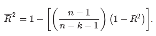
adjusted R-squared

does not automatically increase when another independent variable is added to a regression

R² is strictly greater than adjusted R²

adjusted R² may be negative, whereas the R² has a minimum of zero

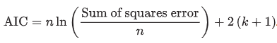
Akaike’s information criterion (AIC)

lower AIC indicates a better-fitting model

Schwarz’s Bayesian information criterion (BIC)

BIC assesses a greater penalty for having more parameters in a model

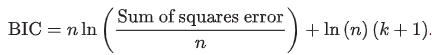
AIC vs BIC

AIC is preferred if the model is used for prediction purposes

BIC is preferred when the best goodness of fit is desired

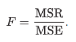
Test whether a variable is significant in explaining the dependent variable’s variation

H₀: b_j = 0 and H_a: b_j ≠ 0

F-distributed test statistic

q is the number of restrictions

How to test for significance

1. Define hypothesis

2. Find critical value

3. Reject the null if calculated statistic exceeds critical value

4. If fail to reject the null i.e. null is correct

general linear F-test

test the null hypothesis that slope coefficients on all variables are equal to zero

Omitted variable bias

• omission of an important independent variable

• If the omitted variable is uncorrelated with X_1, the coefficient for X₁ will still be estimated correctly

Misspecified Regression

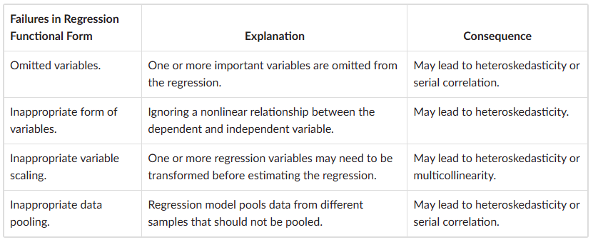
Unconditional heteroskedasticity

error variance is not correlated with the regression’s independent variables - no major problems for statistical inference

Conditional heteroskedasticity

error variance is correlated with (conditional on) the values of the independent variables

• t-statistics will be inflated

• tend to find significant relationships where none actually exist

• more Type I errors (rejecting the null hypothesis when it is actually true)

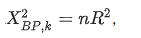
Breusch-Pagan (BP) test

test for conditional heteroskedasticity

heteroskedasticity-consistent standard errors

robust standard errors

• adjust the standard errors of the regression’s estimated coefficients to account for the heteroskedasticity

serial correlation or autocorrelation

regression errors are correlated across observations

• incorrect estimate of the regression coefficients’ standard errors

• no adjustment required if none of the regressors is a lagged value of the dependent variable

• more Type I errors

positive vs negative serial correlation

positive residual for one observation increases the chance of a positive residual in a subsequent observation

a positive residual for one observation increases the chance of a negative residual for another observation

Durbin-Watson (DW) test

• measure of autocorrelation

• compares the squared differences of successive residuals with the sum of the squared residuals

• applies only to testing for first-order serial correlation

• ranges from 0 to 4 (~2 = no autocorrelation, < 2 positive. >2 negative)

Breusch-Godfrey (BG) test

• can detect autocorrelation up to a pre-designated order p, where the error in period t is correlated with the error in period t – p

• n – p – k – 1 and p degrees of freedom, where p is the number of lags

serial -correlation consistent standard errors

adjust the coefficient standard errors to account for the serial correlation

multicollinearity

when two or more independent variables are highly correlated or when there is an approximate linear relationship among independent variables

• impossible to distinguish the individual impacts of the independent variables

• diminished t-statistics, so t-tests of coefficients have little power (ability to reject the null hypothesis)

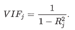
Variance inflation factor (VIF)

• VIF_j > 5 warrants further investigation of the given independent variable

• VIF_j >10 indicates serious multicollinearity requiring correction

correct for multicollinearity

• excluding one or more of the regression variables

• using a different proxy for one of the variables

• increasing the sample size

influential observation

an observation whose inclusion may significantly alter regression results

high-leverage point

data point having an extreme value of an independent variable

outlier data point

data point having an extreme value of the dependent variable

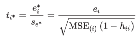
leverage (h_ii) - detecting high-leverage point

• distance between the value of the ith observation of that independent variable and the mean value of that variable across all n observations

• value between 0 and 1

• if an observation’s leverage exceeds

studentized residuals - detecting outliers

• compared to the critical value of the t-distributed statistic with (n − k − 2) degrees of freedom

• |t_i*| > 3 - outlier

• |t_i*| > critical value of t-statistic - potentially influential

dummy variable

• takes on a value of 1 if a particular condition is true and 0 if that condition is false

• to distinguish among n categories, we need n − 1 dummy variables - the category not assigned becomes the “base” or “control” group

Logistic regression (logit)

The natural logarithm (ln) of the odds of an event happening

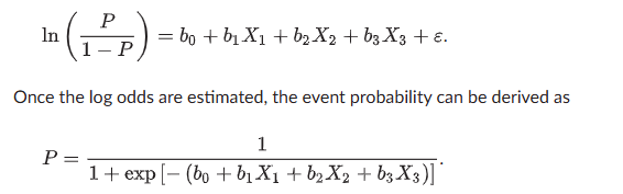
maximum likelihood estimation (MLE) method

• estimates logistic regression coefficients

• a chi-square-distributed test statistic

likelihood ratio (LR) test

• to assess the fit of logistic regression models

• LR = −2 × (Log-likelihood restricted model − Log-likelihood unrestricted model)

• chi-squared with q degrees of freedom

• log-likelihood metric is always negative, so higher values (closer to 0) indicate a better-fitting model

Problems with a time series

• serial correlation in the error term causes estimates of the intercept (b₀) and slope coefficient (b₁) to be inconsistent - independent variable is a lagged variable of the dependent

• The mean or variance of the time series changes over time

log-linear model

ln y_t = b₀ + b₁t + ε_t, t = 1, 2, . . . , T.

Covariance-Stationary

properties, such as mean and variance, do not change over time

• the expected value of the time series must be constant and finite in all periods

• variance of the time series must be constant and finite in all periods

• covariance of the time series with itself for a fixed number of periods in the past or future must be constant and finite in all periods

standard error of the residual correlation

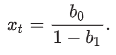
mean-reverting level

root mean squared error (RMSE)

• compare the out-of-sample forecasting performance

• square root of the average squared error

• smallest RMSE is judged the most accurate

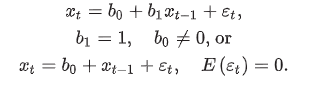
random walk

• value of the series in one period is the value of the series in the previous period plus an unpredictable random error

• error term, ε_t, has constant variance and is uncorrelated with the error term in previous periods

• b₀ = 0 and b₁ = 1

• the expected value of ε_t is zero

• best forecast of x_t that can be made in period t − 1 is x_t−1

• currency exchange rates

• undefined mean-reverting level

• for any period t, the variance of x_t = (t − 1)σ²

• not a covariance-stationary time series, because a covariance-stationary time series must have a finite variance

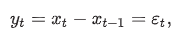
first-differencing

• subtracts the value of the time series in the first prior period from the current value of the time series

• mean-reverting level of the first-differenced model as b₀/(1 − b₁) = 0/1 = 0

• variance of y_t in each period is var(ε_t) = σ²

• variance and the mean of y_t are constant and finite in each period, y_t is a covariance-stationary time series

random walk with drft

• random walk with drift has b₀ ≠ 0, compared to a simple random walk, which has b₀ = 0

unit root

• lag coefficient is equal to 1.0

• all random walks, with or without a drift term, have unit roots

• not covariance stationary

Dickey and Fuller test

• unit root test

• x_t − x_t−1 = b₀ + (b₁ − 1)x_t−1 + ε_t —→ b₀ + g₁x_t−1 + ε_t

• a test of g₁ = 0 is a test of b₁ = 1

• H₀: g₁ = 0; H_a: g₁ < 0

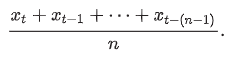
n-period moving average

• to remove short-term fluctuations or noise by smoothing out the time series of sales

• moving average of the current and past n − 1 values

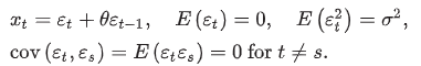
MA(1) - moving-average model of order 1

• moving average of ε_t and ε_t−1

• First: examine the variance of x_t and its first two autocorrelations

• first autocorrelation is not equal to 0, but the second and higher autocorrelations are equal to 0

• MA(1) model has a memory of one period

AR vs MA

autocorrelations of most autoregressive time series start large and decline gradually, whereas the autocorrelations of an MA(q) time series suddenly drop to 0 after the first q autocorrelations

autoregressive moving-average (ARMA) model

• p autoregressive terms and q moving-average terms, denoted ARMA(p, q)

• parameters in ARMA models can be very unstable

• criteria for deciding on p and q for a particular time series are far from perfect

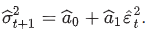
Autoregressive Conditional Heteroskedasticity Models (ARCH)

• If the estimate of a₁ is statistically significantly different from zero, we conclude that the time series is ARCH(1)

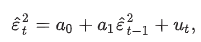
ARCH - predict variance of errors in period t+1

2 time series - one dependent, one independent variable

• test for unit root - DF test

• one of them has a unit root - not covariance stationary; one or more of linear regression assumptions violated; coefficients and standard error inconsistent; coefficient appears significant but is not

• both have a unit root - establish if cointegrated

cointegrated

long-term financial or economic relationship exists between them such that they do not diverge from each other

cointegrated vs not

• not; error term not covariance stationary; some regression assumptions will be violated; regression coefficients and standard errors will not be consistent, and we cannot use them for hypothesis tests

• yes; error term is covariance stationary; regression coefficients and standard errors will be consistent, and we can use them for hypothesis tests; may not be the best model of the short-term relation

cointegration test

• use the critical values computed by Engle and Granger

• fails to reject - not cointegrated

• reject - cointegrated

expected total holding period cost

trading costs = round-trip commission + bid-ask spread

management fees = fee * period