Research Methods

Random Sampling & Stratified Random Sampling

a. Since we are seldom able to measure an entire population, we rely on a random sampling of that population as a representative group from that population. This allows us to infer things about the population, if the sample is truly random. Random sampling is a type of probability sampling. This means it is a method you use to select participants and ensure that every individual/element in the population has an equal chance of being in the sample. Every subject has an equal opportunity for being selected to participate in the study.

For example, one would consider the population of all the university’s athletes: Imagine you have a complete list of all student athletes for your study population—this is your sampling frame. You choose your sample size (N=30), You assign each athlete a unique ID number (say, from 01 to 30 if you have 30 people), and randomly select 30 numbers. You can use a table of random numbers (or a computer-generated list) to select your participants. In this example we want to assume that participant characteristics are reasonably dispersed to increase representative of the larger population.

A truly random sample would sample without replacement. Sampling without replacement increases the probability of the next person/element being selected. Random sampling enhances external validity because it reduces sampling bias, which increases the likelihood of having a representative sample of the population. In turn, allowing researchers to generalize findings to a broader population with greater confidence and making the sample more likely to reflect the characteristics of the larger group.

b. Stratified random sampling is a form of random sampling in which a population is divided into distinct, non-overlapping subgroups—called strata—based on a predetermined, relevant characteristic. For example, dividing a population into groups based on sex (e.g., male and female), age (e.g., 0-18 year olds, 19-60 years olds,), education (e.g., high school diploma, bachelor’s degree, graduate degree), etc.

To conduct stratified sampling: researchers identify the stratification variable (age, gender, etc), identify the sample size needed (N), divide the population into non-overlapping groups/strata, randomly select/sample participants from each stratum. To do this, researchers may create a quota matrix that outlines all possible combinations of these characteristics. Each individual in the sampling frame is sorted into the appropriate cell of the matrix depending on their characteristic. Then, the researchers randomly select participants from each cell, making sure the number of people chosen from each group reflects that group’s actual proportion in the population. For example, if first-year Asian American women make up 5% of the population and the total sample size is 1,000, then 50 people from that group would be randomly selected.

This method is especially useful when researchers want the research sample to accurately reflect the proportions of key characteristics in the study population. It is particularly helpful for studying how trends or variables differ across subgroups and for improving the overall representativeness of the sample. Because individuals within each stratum tend to be more similar (or homogeneous) to one another than to the general population, stratified random sampling reduces sampling variability and increases the precision of population estimates. It also enhances external validity, increasing the likelihood that findings can be generalized to the broader population.

One of the major strengths of this method is that it ensures representation of smaller yet important subgroups that might be overlooked in a simple random sample. This is especially important in studies aiming to compare responses across different demographic groups. However, stratified sampling can be more time-consuming and resource-intensive, as it requires access to detailed demographic information and a complete list of the study population in order to form the strata.

It is most effective when the stratification variable is meaningfully related to the DV. If the stratification variable has little or no correlation with the DV, the benefits of reduced variance and improved representation may not materialize.

An example of stratified random sampling would be using data from the U.S. census to pre-determine the number of different race and ethnic groups in your study so that you can ensure that your sample is representative of the population in the United States. This type of example is commonly used to ensure that assessments such as the MMPI and WAIS have accurate normative samples that are representative of the U.S.

Random Assignment (vs random sampling)

Random assignment is when we assign participants to different groups in an experiment because we want the groups to be an equally random, representative sample of the population. When a participant arrives, the experimenter uses a random procedure, such as a table of random numbers or flipping a coin, to determine if the participant will be in the experimental or control condition. They should not be biased on some characteristic (i.e. age, sex, political belief) and should allocate people to each group in such a way that the probability of each subject appearing in any of the groups is equal. If you randomly assign participants to groups, you assume that personal differences—like intelligence, creativity, or personality traits—will be spread out fairly evenly across groups. For example, if you’re doing a study on art training and some people are naturally more skilled in art (artistic) than others, random assignment increases the chance that both the experimental group and control group will include a similar mix of highly artistic and less artistic people. As a result, the effects of their artistic skill levels should cancel out when the groups’ mean scores on the task are compared. That way, skill level isn't skewing the results. It is important to keep in mind that the larger the sample size, the more likely the groups will, on the average, have the same characteristics. This is important because it helps researchers be confident that any differences in results between the groups were caused by the experimental treatment, not by differences that already existed between the participants. Important for increasing internal validity.

Random sampling refers to how you select individuals from the population to participate in your study and concerns the source of our data (external validity). While random assignment refers to how you place those participants into groups (such as experimental vs. control).

Random sampling increases external validity, while random assignment increases internal validity.

Internal Validity

Refers to the extent to which a study can confidently attribute the observed effects in the dependent variable (DV) to the manipulation of the independent variable (IV), rather than to confounding or extraneous variables. When a study has high internal validity, the results can be interpreted as being caused by the IV. In contrast, when internal validity is low, alternative explanations for the findings remain plausible, making the results uninterpretable. Researchers enhance internal validity by using techniques such as random assignment, control groups, replication, and intent-to-treat analyses. These strategies help ensure that the groups being compared are equivalent at baseline and that changes in the DV can be confidently linked to the IV. Three types of validity are typically examined: content, criterion, and construct validity.

1. Content validity: the degree in which the item contents actually reflect the construct of interest; is the test representative of all aspects of the construct? For example, in the PHQ-9 is it asking all the domains that are included in depression or is it leaving out necessary criteria and topic areas. In order to strengthen content validity, the construct should be well-defined and items generated based on theory and expert judgement, then items statistically examined (e.g., factor analysis) to confirm item content and overlap. Content validity is different from face validity in which the test and construct being measured is discernable to the layperson so they understand what is being measured and feel motivated to complete it. 

2. Criterion validity evaluates how well a test can predict a concrete outcome, or how well the results of your test approximate the results of another test. Is split between both concurrent and predictive validities. Concurrent examines the measure’s score’s relationship to another measure’s score’s taken at the same time while predictive examines whether one’s measurement scores can predict other criterion variables measured at a later time. For example, if a student takes an achievement test and then you use their gpa to see if there is high correlation (concurrent validity). Furthermore, you could also use their achievement test for predictive validity to see how well they might do on a test such as ACT or SAT.

3. Construct validity speaks to whether the measure being examined actually reflects the psychological construct it aims to measure. often used when content and criterion are not available. For example, from what we know about depression, does the PHQ-9 ask relevant information in how we conceptualize depression as a construct? Or is measuring self-esteem, mood, etc.? It is made up of both convergent and discriminant validities. Convergent examines whether the test scores actually correlated with other measure’s test scores with similar constructs to what you are developing (e.g., resilience and grit) while discriminant examines whether the test scores do not correlate with measures it should not theoretically be related to (e.g., resilience and coffee drinking habits). These can be examined using a multi-trait multi-method matrix where correlations with other measures and methods are calculated. Construct validity is also comprised of the test content, its internal structure, its association with other test scores, the psychological processes responsible for test responses, and the test’s consequences.

Compensatory Equalization of Treatment / Threats to Internal Validity

Threats to internal validity are important to control in order to confidently determine that effects on a DV truly result from an IV. Random assignment of participants to groups is integral to increasing internal validity. Further, using control groups, replication studies, and intent-to-treat analyses can be ways to strengthen internal validity.

1) Historical threats refer to events external (outside) to the intervention that occur to all participants in their lives (e.g., natural disaster; global pandemic) that change participants’ responses on the dependent measure or could be attributed to the results (e.g., greater PTSD).

2) Maturation threats refer to naturally occurring processes/changes within participants that occur naturally over time (e.g., growing stronger throughout the year; children become taller as they age). Maturation and history often go hand in hand. People grow/change over time, so an intervention needs to show effects beyond maturation

3) Testing confound confound occurs when taking the pretest affects scores on the posttest independently of the effect of the intervention. The changes in scores may attributed to repeated assessment and familiarity with the test (e.g., people might try to keep their responses consistent by memory across different administrations of a or measure try to “do better” on the posttest than they did on the pretest).

4) Instrumentation: When the measure used to assess the dependent variable changes over time, leading to artificial differences in scores at different points in time, Instrumentation change can take several forms. Mechanical and digital measuring devices can go out of calibration as they are used, resulting in cumulative inaccuracies. (e.g., a timer may begin to run faster or slower with use, especially as batteries weaken). Another form of instrumentation change occurs during the process of coding or categorizing qualitative data; known as observer drift, this change is due to coders becoming less reliable over time. Last cause is a change in the way observers classify participants’ behaviors into categories. The solution to these various forms of instrumentation change is to periodically test any apparatus that might be subject to them, assess the reliability of raters at several points in the coding process, and have different observers code the behavior of interest in different random orders.

5) Statistical regression, also referred to as regression to the mean, threats refer to the phenomenon that occurs when utilizing participants with extreme scores. These extreme scores are often due in part to random error or temporary factors (e.g., someone had a bad day when they took the test). As a result, participants may show improvement (or decline) on a subsequent measure simply because their scores naturally move closer to the mean/average of the population over time—not because of any intervention. For example, you’re doing a study on a new therapy for anxiety, and you only include participants who scored extremely high on an anxiety scale. After the therapy, their scores are lower. That looks like the treatment worked—but regression to the mean might also explain the change. This can create the false impression that a treatment was effective when the change was actually due to statistical regression.

(Regression to the mean = Statistically, an individual who achieves an extreme score on the first testing will probably score closer to the mean on the second testing. The problem here is that you need to make sure the decrease in DV is more likely due to the IV than regression.)

6) Selection bias threats occurs when research participants in the control condition differ in some way from those in the experimental condition and may influence treatment differences in results rather than treatment conditions themselves. These differences are before any experimental manipulation occurs, due to volunteer bias, the use of pre-existing groups in research, and mortality. Random selection helps avoid this

Volunteer bias: a type of selection bias. People who volunteer for research differ on a number of characteristics from those who do not volunteer. For example, volunteers tend to be better educated, of higher socioeconomic status, and more sociable than non-volunteers. To the extent that these characteristics are related to the dependent variable, you cannot be sure that any differences found between the experimental and control groups are due to the independent variable rather than to differences in participant characteristics.

Pre-existing groups: Selection biases can also arise in research conducted in natural settings when researchers must assign pre-existing natural groups to experimental and control conditions. (e.g., employees in a company, rather than individuals). People in pre-existing groups are likely to have common characteristics that can be confounded with treatment conditions when the groups are used as experimental and control groups in research.

Mortality/Attrition threats refer to the loss of subjects when studies take more than one session. Attrition is a direct function of time --> the longer a study goes, the more participants you’ll loss. It can be particularly problematic if there are different rates of attrition across groups. The main thing is the possibility that participants who drop out may share specific characteristics resulting in treatment effects only applying to the “survivors” of the study. Essentially, when participants who drop out differ systematically from those who stay, the remaining sample may no longer be representative, thus affecting the study's ability to accurately assess the relationship between variables. 

7) Diffusion of treatment threats refers to instances in which control groups accidentally receive parts of the intervention, or the intervention group fails to receive all parts; this threat dilutes true treatment effects in the results. When the interventions/conditions of one group accidentally spread to another/control group (e.g., the control group and treatment group talk to each other). When the control group is exposed to the treatment, they may no longer be a true control, as they are receiving some form of the intervention. Diffusion can also lead to resentment or demoralization within the control group, as they may feel disadvantaged compared to the treatment group. Ex: a study investigating the effectiveness of a new teaching method. If the control group learns about the new method from the treatment group (perhaps through shared conversations or observing the treatment group's learning), then any observed improvements in the control group's performance could be attributed to the diffusion of treatment rather than the intended intervention

8) Reactivity threatens the internal validity of research because participants’ scores on measures result from the reactive situation rather than from the effects of the independent variable. Reactivity can stem from two sources: evaluation apprehension and novelty effects. These factors can elicit social desirability response biases, distract people from the research task, and affect physiological responses.

Evaluation apprehension: refers to the nervousness people feel when they believe their behavior is being judged. This concern often leads individuals to act in ways they think will be seen positively, whether in observable behavior or self-report responses. As a result, participants might underreport socially undesirable or private behaviors, such as aggression, prejudice, or certain sexual and health-related habits, and may avoid actions that could embarrass them. This effect is especially strong in the presence of authority figures, like researchers, who are often viewed as having expertise in analyzing behavior. Evaluation apprehension can also distract participants and impair performance, which may threaten the validity of the study.

Novelty effects: Any aspects of the research situation that are new (or novel) to the participants can induce reactivity. These novelty effects stem from participants’ apprehension about dealing with the unfamiliar and paying attention to the novel features of the situation rather than the task at hand. (e.g., being in a laboratory setting, wearing new types of equipment).

External Validity & Generalizability (vs internal validity)

External validity: the extent to which the results of an experiment can be generalized beyond the specific conditions of that experiment to other groups or settings outside of the lab and into the real world. Are the findings of a study specific to the conditions under which the study was conducted, or do they represent general principles of behavior that apply under a wide-ranging set of conditions? Do these findings extend beyond the sample that the research study was conducted on? External validity also requires internal validity to determine that the conclusions in the study are first trustworthy.

External validity consists of both generalizability, or “generalizing across” and ecological validity, “generalizing to”. Generalizability refers to the question of whether the results of a study apply to settings, populations, treatments, or outcomes that were not included in the study. Will the general principles of behavior and theories apply across populations, settings, or operational definitions. For example, if a study on PTSD treatment works in a sample of male combat veterans, generalizability asks whether the same treatment would be effective for civilians, women, or those with PTSD from other causes like domestic violence. Ecological validity refers to the question of whether the results of a study apply to particular settings or populations, such as hospitalized psychiatric patients. High value is placed on the ecological validity of research, which is the degree to which the methods, materials, and procedures used in a study mimic the conditions of the natural setting to which they are to be applied.

To further understand external validity, it can be broken down into three components: structural, functional, and conceptual. The structural component refers to the setting, procedures, and sample characteristics—essentially, how the study was carried out—and is relevant to both generalizability and ecological validity. The functional component assesses whether the psychological processes elicited in the study setting mirror those in the natural environment where the findings might be applied. Finally, the conceptual component considers whether the research questions being addressed are meaningful and relevant to real-world problems. Together, these components help researchers evaluate how confidently study findings can be applied outside the lab.

Considering external validity in research is essential because the interaction between an independent and dependent variable may be influenced by other situational or contextual factors. These include participant characteristics (such as demographics or clinical status), inclusion or exclusion criteria, the setting of the study, and the nature of the intervention or exposure. Such factors can limit a finding’s generalizability to different populations or environments. Subsequent studies are often needed to determine whether the observed effects hold across varied conditions and to examine possible confounding variables or interactions.

When a researcher hopes to increase the external validity of their research, they might hope to increase its generalizability to broader groups (e.g., studies with children to be applicable among teens); however, the nature of applying sample-based findings to a target population means findings may not apply to others without infinitely researching other groups. Overgeneralization can occur when findings from a restricted sample are used without proper replication studies under expanded conditions; for instance, it would be inappropriate to use a drug for people with varied ethnic backgrounds if it had only ever been tested among European individuals.

VS Internal Validity – Internal validity is the extent to which a study successfully rules out or makes implausible alternative explanations for the results, usually by careful study design. In other words, greater internal validity indicates that effects on the DV can be confidently attributed to the IV. Successful internal validity can result from careful control of confounding factors that might have jeopardized interpretation of the results.

Threats to external validity

Threats to external validity might be used as criticisms of most studies but can come across as superficial without plausibility that the factor actually restricts generalizability of the result. For instance, researchers can easily criticize a study by stating the investigator did not examine an effect within an older population.

1) Sample characteristic threats refer to results relying on the demographic or natural characteristics of participants (e.g., undergraduates).

2) Narrow stimulus sampling threats refer to results being limited to the stimulus, materials, or researchers involved, limiting their extension to non-experiment conditions.

3) Reactivity of experimental arrangements and of assessment refer to participants’ awareness that they are part of an experiment that may influence non-experimental generalizability as well as awareness that influences how a participant might respond to questions (e.g., answering favorably).

4) Test sensitization threats refer to participants becoming aware of pre-test assessment procedures that influence or trigger them to respond differently upon follow-up (e.g., greater insight into experiment; “aha! I was asked xx”).

5) Multiple-Treatment interference threats refer to order effects, or the difficulty in ascertaining whether treatment effects result from separate treatments, or the order of conditions given.

6) Novelty effect threats refer to new aspects or environments in an experiment contributing to results rather than the intervention itself (e.g., new therapy setting). 

Power (Type I vs Type II Error)

Statistical power refers to the probability that a statistical test will correctly reject a false null hypothesis (detecting a real effect).s The null hypothesis is the hypothesis that there is no significant difference between specified groups/populations (p < .05) and that any observed difference being due to sampling or experimental error. In other words, Statistical power is the probability that a study will correctly detect a true effect of the independent variable on the dependent variable when one truly exists. This is represented mathematically as 1 - β, where β, or beta, is the probability of making a Type II error. A type II error is failing to reject (or accepting) the null hypothesis when the null hypothesis is indeed false and the alternate hypothesis is true (i.e., there was a finding that was missed). High statistical power is essential for drawing valid conclusions from research because it reduces the likelihood real effects going undetected due to insufficient sensitivity of the study design. High power in a study indicates a large chance of a test detecting a true effect, thus, approximately 80% power is recommended by many researchers. Low power means that your test only has a small chance of detecting a true effect or that the results are likely to be distorted by random and systematic error.

Power is influenced by three main factors: alpha level, effect size, and sample size. When any of these factors increase, power does as well.
(1) the alpha level is typically set at .05. It is known as Type 1 error rate, which refers to rejecting the null hypothesis when it is in fact true. For example, a researcher concludes that the result confirms their hypothesis when the result was actually due to random error.
(2) the effect size, or the the size of the effect that the independent variable has on the dependent variable, and
(3) the sample size.

When the alpha level is decreased (e.g., from .05 to .01), the researcher adopts a more conservative/stricter criterion, requiring stronger evidence to reject the null, or to conclude that an effect is statistically significant. This shift effectively moves the cutoff for significance further into the tail of the probability distribution, making it more difficult to detect true effects. As a consequence, the probability/liklihoood of type II error increases (failing reject a null hypothesis/to detect a real effect), thereby reducing statistical power.

If you increase alpha it will become easier to you make it easier to conclude that there is a significant effect (easier to reject the null hypothesis). Because of this, you reduce Type II error, or the chance of failing to reject the null when the null is actually false. Therefore, power increases because it becomes easier to detect a true effect and avoid missing it (reducing Type II errors). However, the trade-off is that you also increase the chance of making a Type I error — wrongly rejecting the null hypothesis when the null is true (it is not significant but you reject anyways b/c you believe it is true.).

If we increase effect size (= increase of distance between the centers of distribution) probability of Type II error (beta) will decrease causing power to increase.

As sample size increases, our estimation of population mean and SD gets better and variability in the sample means goes down causing power to increase as sample size increases.

Low power leads to misleading conclusions, overestimation of effect sizes, poor replicability, and ethical concerns. Conducting a power analysis with 3 of the following 4 things: effect size, alpha, power, and number of participants, can aid in reaching statistical power.

Type I VS Type II Error

1. Type I error refers to rejecting the null hypothesis when it is in fact true. For example, a researcher concludes that the result confirms their hypothesis when the result was actually due to random error. Type I error is represented by alpha as the probability of this occurring. Alpha is usually arbitrarily set prior to conducting hypothesis testing (e.g., 0.05, 0.01). By reducing alpha and the probability of a type I error, we are increasing the probability of committing a type II error. A type II error is failing to reject (or accepting) the null hypothesis when the null hypothesis is indeed false and the alternate hypothesis is true (i.e., there was a finding that was missed). This is represented by beta. For example, with an alpha = .01, the beta = .92. 

2. Type I/Type II error are important because depending on the study you are running it may be important to reduce alpha, thereby increasing your odds of making a type II error, but decreasing your odds of making a type I error. For example, a study might explore the effects of a drug with extreme side effects but impactful benefits; reducing alpha to 0.01 might help researchers err on the side of caution so they do not disperse a drug that does not truly cure the disease and unnecessarily give dangerous side effects (Type I error). 

Demand characteristics and experimenter expectancy effects

Demand characteristics and experimenter expectancy effects are threats to construct validity (the extent that your measure- measures what it is intended to) due to their impact on results.

1. Demand Characteristics: Because individuals naturally attempt to understand what is happening to them and the meaning of events, participants will frequently try to understand the nature of the research and hypothesize about its goals. In doing so, participants may attempt to adjust the outcome of the research as a form of reactivity. Participants might make assumptions based on the information provided through sources of information (such as instructions, procedures informed consent) or by deriving information from structure of the research task/procedures. These subtle cues/demand characteristics can make participants aware of what the experimenter expects to find or how participants are expected to behave. This can change the outcome of an experiment because participants will often alter their behavior to conform to expectations. When participants think they know what the researcher is studying, they may act in a way that supports the hypothesis (the “good participant” role), act to contradict it (the “negative participant” role), or disengage entirely (the “apathetic participant” role). Each of these responses can undermine internal validity because the outcomes may reflect participant expectations or motivations rather than the true effect of the independent variable.

Example: Some participants were informed of the purpose of the study was to see the treatment effects (reduced symptoms) of a menstrual cycle pill, and were told that the researchers wanted to look at menstrual cycle symptoms. Both were given placebo pills, however, the group that were informed of the purpose of the study were significantly more likely to report negative premenstrual and menstrual symptoms than participants who were unaware of the study's purpose.

Demand characteristics can be controlled by:

1) Reducing cues to minimize any hints in the research procedures that might lead participants to guess the study’s hypothesis and alter their behavior accordingly. This can be done by avoiding obvious manipulations, using between-subjects designs instead of within-subjects when possible, piloting studies to check for unintended cues, and sometimes using deception—ethically and with debriefing. (e.g., To reduce demand characteristics in a study on ageism, researchers might avoid showing participants both older and younger faces in a within-subjects design. Instead, they use a between-subjects design where each participant only sees one age group.)

2) Increasing motivation of participants by reminding them that their participation is voluntary (can leave at any time) can lower evaluation apprehension and reduce the chance they’ll act as “good” or “negative” participants.

3) Incorporate “fake good” role-playing procedures to estimate true versus purposefully fake participant responses

4) Separating the dependent variable from the study (e.g., deception practices that allow participants to believe the study has ended).

2. Experimenter expectancy effects occur when experimenters’/investigators’ expectations of participant responses result in behaviors, facial expressions, or attitudes (changes in voice, posture, facial expression, delivery of instructions) that affect participants’ responses and how they perform. which biases the data/ This can be unintentional, or it can be intentional b/c experimenters hope to find data that support their hypotheses, or they hope that early detected patterns will result in later predicted data patterns.

   These can result in 1) biased observations, in which hopes and expectations might result in biased ratings (e.g., expecting female participants to be emotional results in greater emotion ratings), or 2) influencing participant responses by treating participants differently based on experimenter assumptions (e.g., nonverbal or verbal feedback to correct answers). Experimenter expectancy effects can be reduced by utilizing detailed scripts, masking conditions from the experimenters, disallowing snooping for patterns in data, using double blind studies in which the experimenter does not know which group or condition the participant is in.

   Example: The researcher may respond to participants by nodding their head, using facial expressions or body language that may influence how the participant answers or responds to the experiment.

Between-subjects versus within-subjects designs

1. Within-subjects designs, or “repeated measures designs",” are when each participant takes part in both the experimental and control conditions so that the effects of participant variables are perfectly balanced across conditions.. Participants might be tested pre- (baseline) and post-treatment, be placed in both the experimental and control conditions, or tested repeatedly across time points.

   Within-subjects case study designs include baseline assessment or their existing level of performance, continuous assessment typically multiple times a week of the same subject, examine pattern and stability of performance, and use of different phases of baseline and intervention. From a within-subject experimental design, one can have an ABAB design where A = baseline and B = treatment (which is applied after a stable baseline has been established), A = return to baseline and removal of treatment. This can account for different treatments. For example. a person measuring their sadness each day for one week, then starting an intervention like exercising each day, recording their sadness each day, then the next week recording sadness but not working out, then the next week recording their sadness and working out again. This allows them to compare to their baseline sadness from week 1 what the effect of exercise is on their sadness level.

   Pros: This design is beneficial in that characteristics among individuals should remain the same across conditions (experimental and control), which reduces error variance and increases the likelihood of detecting real effects (i.e., more statistical power). Since each participant experiences all conditions, fewer total participants are required to achieve the same statistical power as a between-subjects design.

   Cons: However, within-subjects designs are prone to order effects such as: practice (participants improve through repetition), fatigue (participants become tired or bored), carryover (effects of one condition linger and affect the next), and sensitization effects (exposure to one condition changes how participants react to the next, sometimes leading to reactivity or demand characteristics), due to repeated testing. Another disadvantage are the potential for demand characteristics (i.e., When participants experience multiple conditions, they may guess the purpose of the study and alter their behavior to align with or oppose perceived expectations).

2. Between-subjects designs, or “independent group designs,” are studies in which different groups of participants undergo different aspects of an experiment, typically only receiving one condition. Participants would be tested in either the control or experimental conditions and are usually randomly assigned to reduce error and confounding effects. Between-subjects designs can include pretest-posttest control groups (4) or intervention/control groups (3). An example of a between subjects pre-post design would be if one randomly assigned group was given a pre test, then CBT treatment for insomnia, then a post test measure. The comparison group would also be randomly assigned, undergo a pre-test, no intervention, then a post-test. Comparison between groups would reveal information about the effectiveness of CBT-i.

   Pros: Each participant is exposed to only one condition, so there's no risk of practice, fatigue, carryover, or sensitization effects, reduced demand characteristics.

   Cons: To achieve adequate power, you need more participants since each person only provides data for one condition. Even with random assignment, groups may differ in meaningful ways (e.g., one group could end up with more high-performing individuals), which introduces variability and can obscure real effects.

The word “between” means that you’re comparing different conditions between groups, while the word “within” means you’re comparing different conditions within the same group.

Manipulation Check

A manipulation check is a crucial step in experimental research used to verify whether the independent variable was successfully manipulated as intended. It serves as a form of construct validation, confirming that participants in different experimental conditions experienced the expected differences in the independent variable. For example, if a study is designed to induce stress, a manipulation check would assess whether participants in the high-stress group actually reported experiencing more stress than those in the low-stress or control group. These checks can be implemented during or after data collection, either through direct measurement (e.g., self-reports or behavioral indicators) or post-experimental interviews where participants reflect on their experiences. Manipulation checks also help establish discriminant validity, ensuring that the manipulation only affects the targeted construct and not unrelated variables. Without this step, researchers risk misinterpreting null results—if a manipulation fails but no difference is observed, it’s unclear whether the independent variable truly has no effect or if the manipulation simply didn’t work. Therefore, manipulation checks are essential for interpreting findings and for ensuring the internal validity of an experiment.

Researchers may also include objective methods such as observer ratings or informant reports, and ensure fidelity through treatment manuals, staff training, and ongoing supervision. A successful manipulation check allows researchers to conclude that participants accurately perceived and engaged with the independent variable, thereby increasing internal validity and supporting more confident inferences about causal relationships between variables. Conversely, if a manipulation check fails, it may signal a need to refine the intervention or reevaluate the theoretical assumptions behind it.

Waitlist Control

Control group is a group that is ideally the same as the experimental group but doesn’t get the treatment or experimental manipulation. A control group is used to reduce the chance of threats to internal validity (i.e. history, maturation, selection and testing). In waitlist control groups, treatment is withheld from the control group for a period of time after which they receive treatment, typically they serve as the control group until the experimental group finishes course of treatment. For this group to be most effective, subjects need to be randomly assigned.

There are 3 features of wait-list controls

(1) if pretest is used, there must be no treatment between 1^st and 2^nd assessment period

(2) the time period from first to second assessment must correspond to the time period pre-post assessment of the treatment group

(3) wait-list controls complete the pre- and posttest assessments. T

Wait-list control groups are easier to obtain than no-treatment control groups as they are simply delayed rather than withheld assistance; however, wait-list control groups need to have extra considerations for their unique needs for treatment, providing other resources, and the severity of the condition. Additionally, it is difficult to ascertain maturation and history effects for this group because natural changes over time may be large or small.  There may also be ethical issues if an individual is in need of immediate treatment and the long term impact of factors like history cannot be evaluated.

 

o   Here is how a waiting-list control group is diagrammed:

R	O	X	O2
R	O3		O4	X	O5

X= treatment or independent variable

O=observation (pre/post teat) of independent variable

Independent Variable vs Dependent Variable

The IV contains conditions that are varied or manipulated to produce/cause changes or differences among conditions/other variables in a study. Studies are often based on hypotheses framed as “if-then” statements—for example, if participants receive a certain treatment (IV), then their behavior or response (dependent variable) will change in a specific way. The “if” part refers to the independent variable, which is expected to cause or influence a change in the dependent variable.

There are three main types of independent variables:

1. Environmental variables involve manipulating the environment or situation—for example, assigning participants to an experimental or control group, changing the room lighting, or introducing a loud noise. These are things done to, with, or by the participant.

2. Instructional variables involve changing what participants are told or what they believe about the task. For instance, participants might be told that a test measures intelligence or creativity, even if the task is the same in both conditions.

3. Subject (or individual difference) variables refer to pre-existing characteristics of participants, like gender, race, personality traits, or clinical diagnoses. While these cannot be manipulated by the researcher, they can still be treated as independent variables in certain types of research designs.

The researcher typically controls the independent variable and they can be described in different ways:

• Quantitative (measured in numerical values, like age or number of hours slept),

• Qualitative (categories, like treatment type),

• Discrete (distinct groups or categories, like “yes” or “no”),

• Continuous (variables that can take on a wide range of values, like stress level on a scale of 1 to 100).

The dependent variable (DV) is the outcome that researchers measure to determine whether it has been influenced by changes in the independent variable (IV). In experimental research, the goal is to assess whether manipulating the IV causes a change in the DV—such as changes in behavior, performance, emotion, or physiological response. For example, in a study testing whether sleep affects memory, the amount of sleep is the IV, and memory performance (the DV) is measured to assess its effect.

In correlational studies, where variables are not manipulated but simply measured, the DV represents the effect or outcome the researcher hopes to predict or explain based on its association with other variables. Although researchers look for relationships between IVs and DVs, especially in correlational research, it's important to remember that correlation does not imply causation, and relationships observed cannot prove that one variable causes the other.

Dependent variables are often continuous, meaning they can take on a wide range of values (e.g., test scores, anxiety levels), but they can also be categorical (e.g., yes/no responses, diagnostic outcomes). The validity and sensitivity of the DV are critical—if a DV is poorly chosen or measured, it can weaken the study’s ability to detect meaningful effects.

Counterbalancing

Counterbalancing is a method used in experimental design to control for order effects—that is, the possibility that the order in which treatments or conditions are presented might affect the results. Imagine you're testing two different treatments (A and B) to see which works better. If everyone gets A first, then B, you can't be sure if B looks better just because it came second—maybe participants were more tired, more experienced, or more motivated the second time. That’s called an order effect, and it can confound (mix up) your interpretation of which treatment actually worked better.

Counterbalancing mixes up the order in which participants receive treatments. This way, any effects caused just by the order, such as practice effects where participants perform better the second time after being exposed to it previously, are spread out evenly across conditions, making it easier to isolate the actual effect of the treatment itself.

• Simple counterbalancing For 2 conditions (A and B), would mean half the participants undergo the experimental condition first and the other half undergo the control condition first. This procedure is designed to spread practice effects evenly across the conditions so that they cancel out when the conditions are compared.

  • Group 1: A → B

  • Group 2: B → A

For experiments with two conditions, counterbalancing is straightforward: half the participants experience Condition A first and Condition B second, while the other half experience condition B first, then A. This ensures that any practice or fatigue effects are balanced out across conditions. However, as the number of conditions increases, the number of possible sequences grows factorially For example, three conditions require six orders, four require 24, and five require 120. To manage this complexity, researchers often use partial counterbalancing methods such as Latin square designs, which ensure that each condition appears equally often in each ordinal position, though they may not perfectly balance every possible sequence of conditions. An example of Latin Square design would be to administer 123 to one group, 231 to the other, and 312 to the last group.

In addition to balancing order, counterbalancing can help distribute carryover effects, but it is also advisable to include washout periods between conditions when residual effects from one condition might influence another. For example, in pharmacological studies, participants might complete different drug conditions on separate days to allow the effects of the first drug to dissipate before the next session.

Mediation vs Moderation

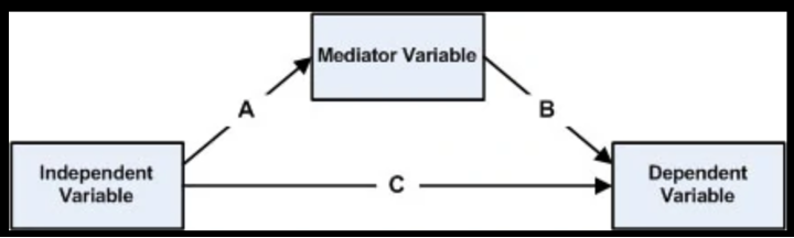
Both mediation and moderation, as outlined by Baron and Kenny (1986), involve a third variable that influences the relationship between an independent variable (IV) and a dependent variable (DV), but they do so in fundamentally different ways. Mediation occurs when the third variable explains why or how an IV affects a DV. In this case, the mediator accounts for the causal pathway from the IV to the DV. For us to claim a mediation effect the first step is to show a significant relationship between independent variable and the mediator (A) and then show a significant relationship between the mediator and the dependent variable (B) and then a significant relationship between the IV and DV (C). However, others have argued that these requirements for mediation result in very low power. Thus, the final step in proving mediation is that once the mediator and independent variable are used simultaneously to predict the dependent variable, then the significant path between the independent and dependent variable is now reduced, if not insignificant. Therefore, mediation tests the causal chain X leads to change in mediator which leads to change in Y and explains why X affects. For example, SES (socioeconomic status) may predict parental education levels —> Parental education levels predict child reading ability. So, parental education levels act as a mediator b/c they help explain how or why SES influences child reading ability. Simple, three-variable mediational hypotheses like this can be tested using the causal steps strategy and multiple regression analysis. One way to statistically assess mediation is by computing the indirect effect, which my multiplying coefficient a by coefficient b (a × b), where a is the unstandardized regression coefficient from the relationship between the IV and mediator, and b is the coefficient from the mediator to the DV (controlling for the IV). This product (ab) is then divided by its standard error in a Sobel test, andiIf ab is statistically significant, one can conclude that that mediator variable mediates the relationship between IV and DV.

Moderation: In contrast, moderation occurs when the strength or direction of the relationship between an IV and DV changes depending on the level of a third variable. A moderator answers the question of when, for whom, or under what conditions an effect occurs, rather than explaining why. For example, the effect of parental education on child reading ability may be moderated by the child’s access to books at home—meaning that parental education predicts stronger reading skills only when book access is high. Unlike mediation, moderation does not assume a causal chain but rather an interaction, often tested using regression analysis with interaction terms. In sum, mediators explain effects, while moderators qualify them

Standardized Scores

Standardized scores are important because they allow us to calculate the probability of a score occurring within a normal distribution, which is fundamental in inferential statistics. By converting raw scores into a common metric, standardized scores also enable us to compare scores that originate from different distributions or tests with varying scales. Standardization involves converting raw data through linear transformations, which preserve the relative differences between scores while rescaling them to a standardized format. In other words, standardized scores are simply transformed observations that are measured in standard deviation units. For example, a z-score indicates how many standard deviations a particular observation lies above or below the mean of its distribution. Because z-scores transform data to have a mean of zero and a standard deviation of one, they create a standardized scale that facilitates direct comparisons across different datasets or measures. This standardization is crucial when conducting inferential statistical tests, where assumptions about normality and comparable scales often apply. For instance, IQ scores are transformed from raw test results to a distribution with a mean of 100 and a standard deviation of 15. This transformation allows an IQ score, such as 120, to be translated into a z-score indicating how many standard deviations it lies above the mean. Given that IQ scores approximate a normal distribution, this z-score can then be converted into a percentile rank; for example, an IQ of 120 corresponds roughly to the 91st percentile, meaning the individual scored better than approximately 91% of the population.

In addition to z-scores, there are other commonly used standardized scores designed for specific contexts. For instance, scaled scores typically have a mean of 10 and a standard deviation of 3 and are often used in intelligence testing to make interpretation more intuitive. T scores, which have a mean of 50 and standard deviation of 10, are commonly used in psychological assessments to convey how an individual’s score compares to a normative group. Together, these standardized scores provide versatile tools for interpreting individual performance relative to a broader population or distribution.