BE501 - Economics I: Microeconomics (Midterm)

Lectures 1-6

Microeconomics

Microeconomics

Analysis of markets and the interplay between consumers and producers.

Fundamental assumptions

1. Resources are scarce.

2. Agents do as well as possible given the constraints they face.

Two types of economic analysis

1. Positive analysis: Testable hypotheses about what happens if different event occur or actions are taken.

2. Normative analysis: Gives recommendations. How something should be. Depends on values/preferences and on positive economics/analysis.

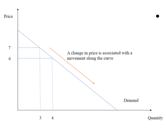
Demand

The quantity that buyers wish to purchase.

“Law of demand”

Effect on demand of changes in the price of the good.

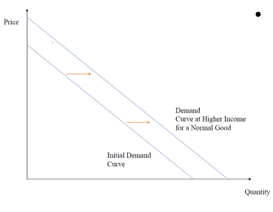
Effect on demand of changes in income

Increase for normal goods and decrease for inferior goods.

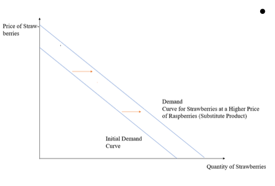
Effect on demand of changes in price of other goods (substitutes)

Demand for good increases when price of substitute increases.

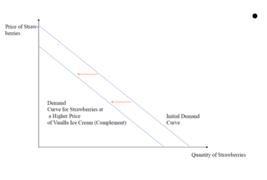
Effect on demand of changes in price of other goods (complements)

Demand for good decreases when price of compliment increases.

Inverse demand function

Price as a function of quantity. E.g. P=5-2Q.

Supply

Quantity that sellers are willing to sell.

What supply depends on

• Price

• Production costs

• Number of sellers

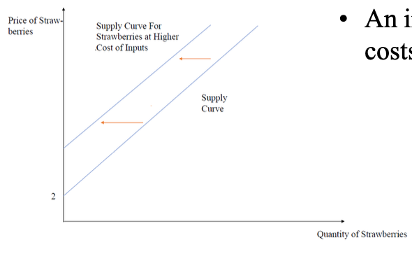
Supply with an increase in costs of inputs

Decreased supply.

Equilibrium

Quantity demanded = Quantity supplied

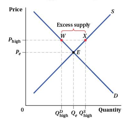
Excess supply

Price is higher than equilibrium.

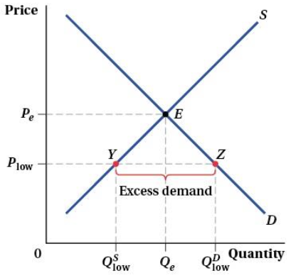
Excess demand

Price is lower than equilibrium.

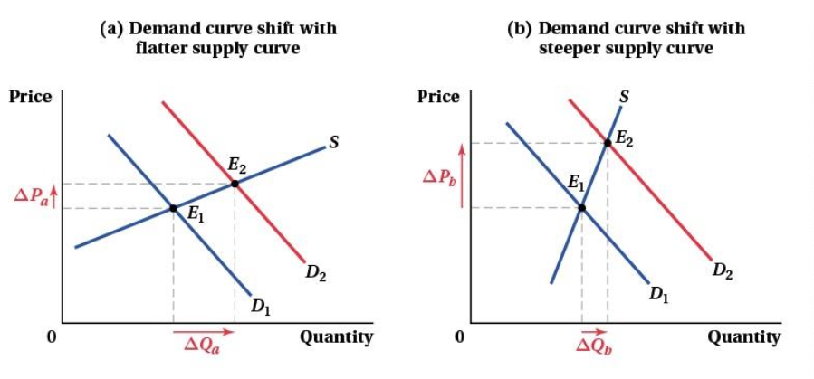
Two parameters that determine the magnitude of change in equilibrium price and quantity

1. Size of the shift

2. Slope of the curves

   • Demand shifts: Slope of supply curve determines the size of change.

   • Supply shifts: Slope of demand curve determines the size of change.

Assumptions regarding preferences

• Completeness: We can rank all bundles

• Transitivity: If A>B and B>C => A>C

• Non-satiation: More is better

  • Decreasing marginal utility

Decreasing marginal utility

The more you have of a good, the less you value additional units of that good.

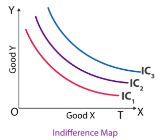
Indifference curve

Connects all combinations of goods that the individual values the same (same utility). Slope indicates how individual is prepared to substitute between the different goods.

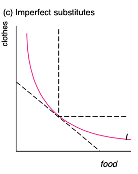
Imperfect substitues

Two goods that replaces each other, but has significant differences. Preferably the individual wants both goods.

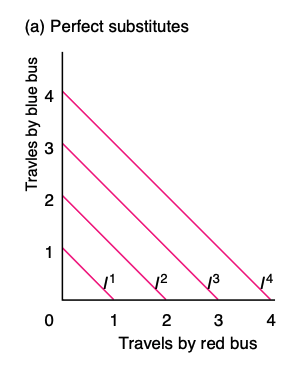
Perfect substitutes

Two goods that replaces each other, and can be used in the same way.

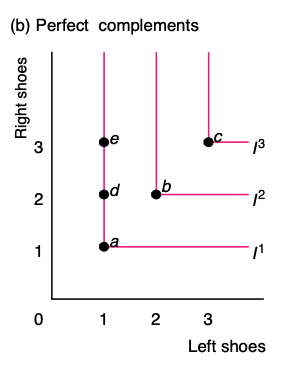
Perfect complements

The individual always wants to consume both goods in the same proportion.

Marginal rate of substitution (MRS)

Slope of indifference curve.

Determines how an individual is willing to trade off one good against another, and still be equally well off.

For imperfect substitutes, MRS depends on where it is evaluated.

Budget constraint

Determines which choices the individual can afford.

Marginal rate of transformation (MRT)

Slope of the budget constraint.

How to reach maximised utility

Choose consumption such that utility is maximised under the budget constraint.

Indifference curve is tangent to budget line. (MRS=MRT).

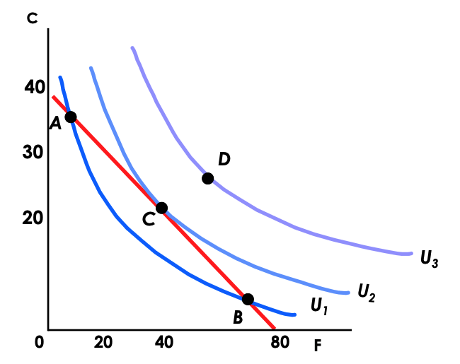
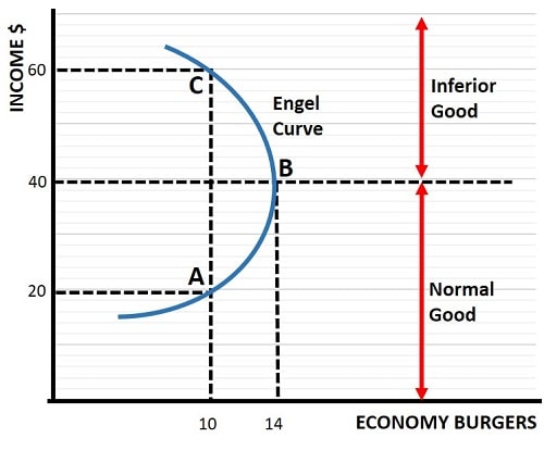
Normal goods

Income increases => Demand increases

Inferior goods

Income increases => Demand decreases

Good can be normal at low incomes and inferior at higher incomes.

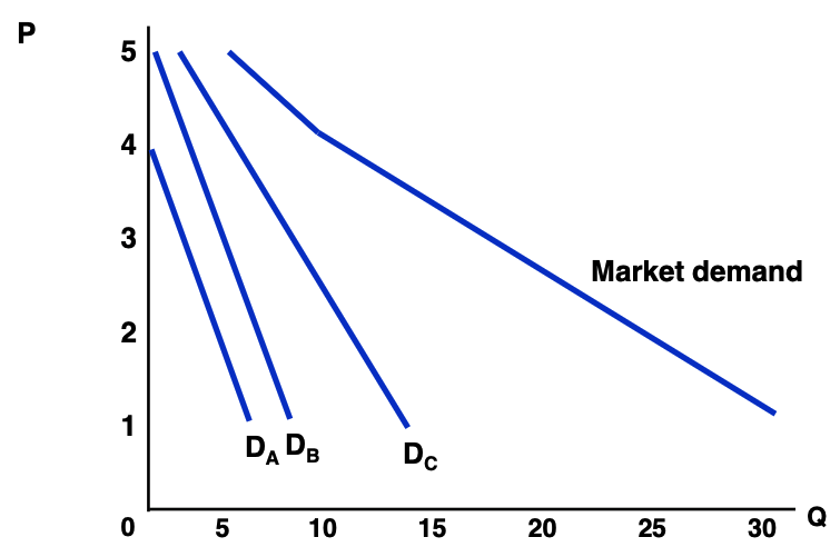
Market demand

Total quantity of good consumers are willing and able to purchase at a given price.

Elasticities

The sensitivity of demand or supply to prices or incomes.

Percentage change in one variable (e.g. quantity) divided by the percentage change in another (e.g. price).

Price elasticity of demand

(%change in quantity demanded)/(%change in price)

E^D=(∆Q^D)/(∆P)*(P/Q^D)

Large price elasticities of demand => Consumers can easily substitute good when price increases.

Less price elasticities of demand => Consumers have fewer options for substitution.

Price elasticity of supply

(%change in quantity supplied)/(%change in price)

E^S=(∆Q^S)/(∆P)*(P/Q^S)

Large price elasticities of supply => Easy for suppliers to vary their amount of production/quantities as price changes.

Low price elasticities of supply => Difficult for suppliers to increase production/quantity as price increases.

Income elasticity of demand

The ratio of the percentage change in quantity demanded to the corresponding percentage change in consumer income. How responsive demand is to income changes.

E_I^D =( ∆Q^D / ∆I ) * ( I / Q^D )

Cross-price elasticity

The ratio of the percentage change in good X’s quantity demanded to the percentage change in the price of another good Y.

E^D_XY = ( ∆Q^D_X / ∆P_Y ) * ( P_Y / Q^D_X )

E^D_XY > 0 => Consumers demand higher quantity of X when price of y increases. I.e. X is a substitute of Y.

E^D_XY < 0 => Consumers demand lower quantity of X when price of Y increases. I.e. X is a compliment of Y.

Factors of production

• Capital

• Labor

• Raw materials

  • Intermediate inputs (goods & services used in production process rather than for final consumption)

Marginal product of labour (MP_L)

How much the volume produced increase if more labour is used (capital is kept constant).

MP_L = ∆Q / ∆L

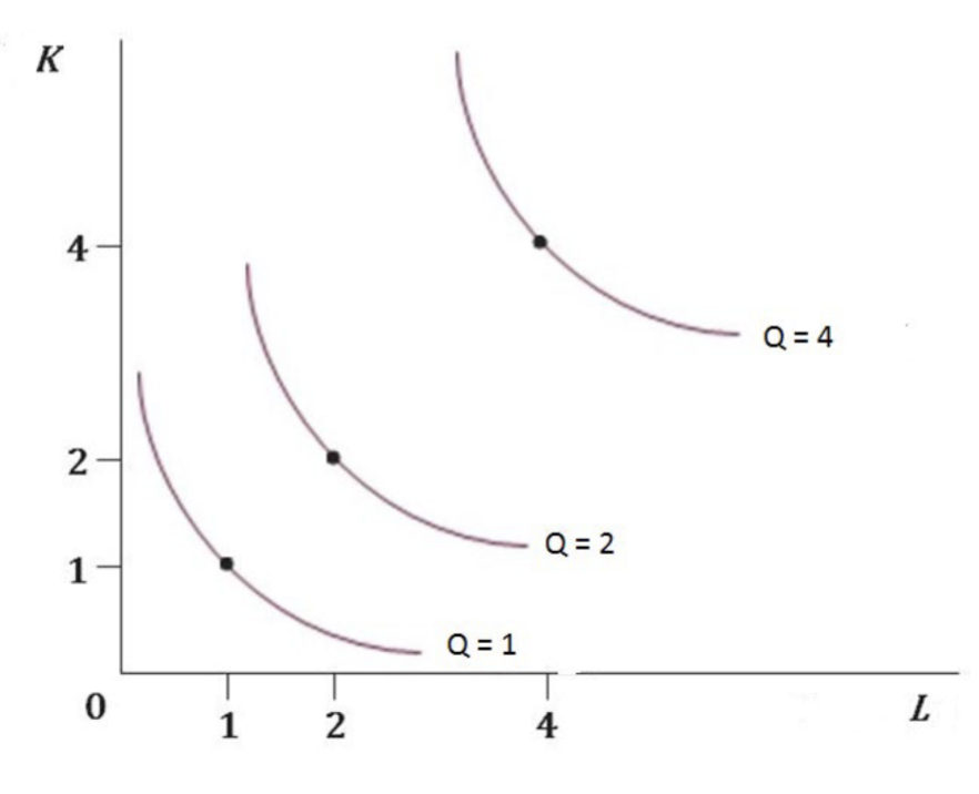
Isoquant curve

A curve drawn through the set of points at which the same quantity of output is produced while changing the quantities of two or more inputs (e.g. capital and labour).

Marginal technical rate of substitution (MRTS)

The slope of the isoquant.

MRTS_LK = - ∆K / ∆L

The rate at which the firm can trade input K (capital) for input L (labour), holding output constant.

Returns to scale

How much more that is produced if we use more of all inputs.

Constant returns to scale

When quantity produced doubles if all inputs doubles.

Decreasing returns to scale

When production/output increases by less than the increase in inputs.

Increasing returns to scale

When production/output increases by more than the increase in inputs.

Productivity

Technological and organizational changes can lead to higher quantities produced, with the same amount of inputs. E.g term A in following production function:

Q = A * f(K, L)

Cost (two inputs)

C = WL + RK

C = Cost

W = Wage

L = Labour

R = Rental rate

K = Capital

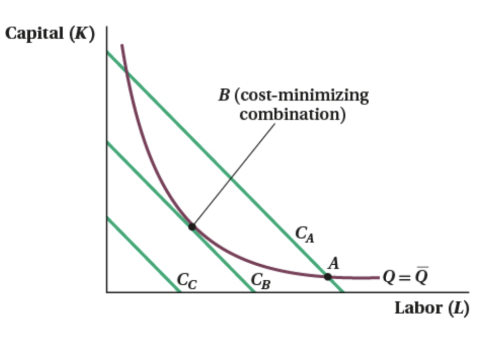
Isocost

Combinations of capital (K) and labour (L) that give the same cost (C).

Cost minimization

The point where the isoquant is tangent to the isocost.

( MP_L / MP_K ) = W / R

Economic cost

Economic cost = Opportunity cost + Accounting cost

Opportunity cost = The cost of not using a resource in the best alternative way.

Accounting cost = Monetary costs

Different types of costs

• Fixed costs (FC): Don’t depend on quantity.

• Marginal cost (MC): Increase in costs associated with producing one more unit. MC = C’(q)

• Average total cost (ATC): Average cost per quantity. ATC = C(q)/q

• Variable cost (VC): Total cost excluding fixed cost. VC = C(q) - FC

  • Average variable cost (AVC): Average variable cost per quantity. AVC = ( C(q) - FC ) / q

Profit

Revenue - cost

Profit maximizing quantity

R’(q) - C’(q) = 0

MR - MC = 0

Perfect competition

A market or industry in which many firms produce an identical product and there are no barriers to entry.

Individual firm is a price taker (they set the price to the market price)

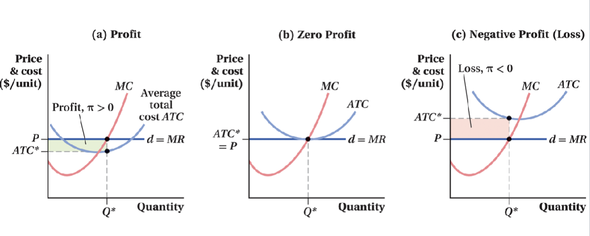
Measuring profit (area calculation)

π = Q * (P - ATC)

Q* = Quantity where P=MC
P = Market price
ATC = Average total cost where Q*

π > 0 => Profit

π < 0 => Loss

π = 0 => Zero profit

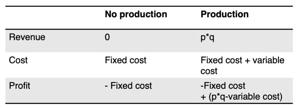
Can it be worth producing even though the firm makes a loss?

Short run: Produce if p ≥ AVC.
Because the fixed cost will in the short run reduce the profitability more.

Long run: Produce if p ≥ average total cost.
Because the fixed cost will be have a reduced impact on profitability in the long run.

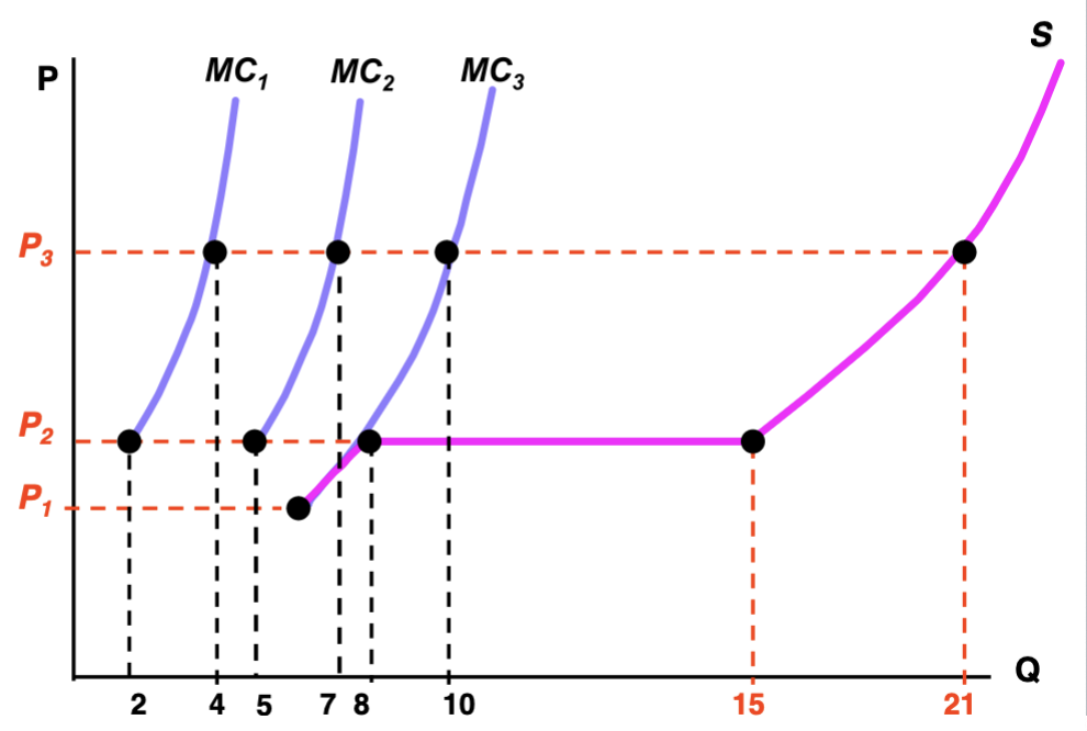
Market supply

The sum of the individual firms’ supply.

Demand/Supply Choke Price

The price at which quantity demanded/supplied is zero; the vertical intercept of the inverse demand/supply curve.

Luxary good

A good with income elasticity greater than 1.

Consumption bundle

A set of goods or services a consumer considers purchasing.

Feasible bundle

Any combination of goods on or below the budget constraint that the consumer has the income to purchase.

Infeasible bundle

Any combination of goods above or to the right of the budget line that the consumer cannot afford to purchase.

Corner solution

A utility maximizing bundle located at the “corner“ of the budget constraint where the consumer purchases only one of the two goods.

Interior solution

A utility maximizing bundle that contains positive quantities of both goods.

Necessity good

A normal good for which income elasticity is between 0 and 1.

Income expansion path

A curve that connects a consumer’s optimal bundles at each income level.

Engel curve

A curve that shows the relationship between the quantity of a good consumed and a consumer’s income.

Short run

The period of time during which one or more inputs into production cannot be changed.

Long run

The amount of time necessary for all inputs into production to be fully adjustable.

Fixed inputs

Inputs that cannot be changed in the short run.

Variable inputs

Inputs that can be changed in the short run.

Diminishing marginal product

The reduction in the incremental output obtained from adding more and more labor.

Expansion path

A curve that illustrates how the optimal mix of inputs varies with total output.

Sunk cost

A cost that, once paid, cannot be recovered.

Specific capital

Capital that cannot be used outside of its original application.

Sunk cost fallacy

The mistake of letting sunk costs affect forward-looking decisions.

Economies of scale

Total cost rises at a slower rate than output rises.

Diseconomies of scale

Total cost rises at a faster rate than output rises.C

Constant economies of scale

Total cost rises at the same rate as output rises.

Long run competitive equilibrium

The point at which the market price is equal to the minimum average cost and firms would gain no profits by entering the industry.E

Economic rent

Returns to specialized inputs above what firms paid for them.

Hyperbolic discounting

The tendency of people to prefer immediate payoffs to later payoffs, even if the later payoffs is much greater.

Endowment effect

The phenomenon whereby simply possessing a good makes it more valuable; that is, the possessor must be paid more than they would have paid to buy it in the first place.

Loss aversion

A type of framing bias in which a consumer chooses a reference point around which losses hurt much more than gains feel good.

Anchoring

A type of framing bias in which a person’s decision is influenced by the specific pieces of information given.M

Mental accounting

A type of framing bias that occurs when people divide their current and future assets into separate nontransferable portions, instead of basing purchasing decisions on their assets as a whole.