S1 Aggregate Supply and the AD-AS Model

What are the two channels through which the Price Level interacts with Aggregate Expenditure to give an AD curve?

Wealth Channel: Through consumption's dependence on non-bank private sector (nbps) wealth.

Competitiveness Channel: A change in the home price level ceteris paribus changes the real exchange rate, affecting competitiveness.

How do Keynes, Milton Friedman, and Franco Modigliani differ in their views on consumption?

Keynes: Consumption depends on current disposable income.

Friedman & Modigliani: Consumption depends on permanent income or lifetime income rather than just current income.

Parents may save today for future consumption or bequests.

Saving adds to the stock of nominal financial wealth (A).

Accumulated assets can fund “big-ticket” purchases (e.g., car, holiday, or school fees).

How does the price level affect non-bank private sector (nbps) wealth, and what distinguishes inside and outside wealth?

Effect of Price Level:

NBPS wealth (A£) includes cash, bank deposits, and bonds.

As P (price level) rises, real wealth falls since A£/PA£ / PA£/P decreases.

Cash & bank deposits = ~16% of NBPS wealth.

Outside Wealth:

Wealth from external sources (e.g., land, foreign investments).

Represents net positive value, not offset by internal liabilities.

Inside Wealth:

Assets and liabilities created within the economy (e.g., loans, stocks).

Net across the economy is zero (one’s asset = another’s liability).

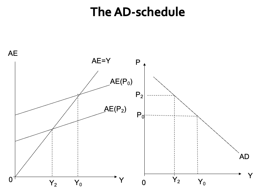
How does the price level (P) affect consumption (C) and the AE-line in real terms?

Consumption Function: C=f(Yd,A£/P)

C rises (falls) as disposable income (Yd) and real wealth (A£/P) rise (fall).

Effect of Price Level (P):

If P rises → Real wealth (A£/P) falls → C falls → AE-line shifts downwards.

If P falls → Real wealth (A£/P) rises → C rises → AE-line shifts upwards.

Outcome:
A rise in P reduces output as AE shifts down.

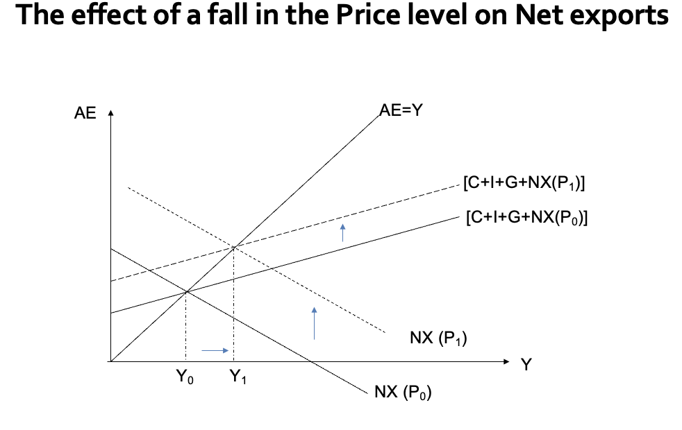
How does a change in the domestic price level (P) affect AE through the net export function and the competitiveness channel?

Net Export & Competitiveness Channel:

When P falls, domestically produced goods become cheaper in foreign markets compared to foreign goods.

Foreign goods become relatively more expensive in domestic markets (assuming a constant exchange rate).

Competitiveness:

Improved price competitiveness causes:

Domestic consumers to buy more domestic goods.

Foreign consumers to increase purchases of domestic exports.

Exchange Rate Note:

E = Foreign price of domestic currency (e.g., $/£).

A rise in E: £ appreciates, $ depreciates.

Result:

Both the NX-line and AE-line shift upwards as P falls (e.g., P0→P1).

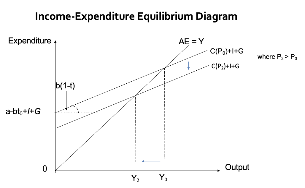
What are the total effects of an exogenous change in P?

The total effect of a rise (fall) in P on AE:

1. is to reduce (raise) consumption via the fall (rise) in NBPS outside wealth, and

2. to reduce (increase) NX as domestic competitiveness declines (improves).

Both of these effects operate in the same direction and so a rise (fall) in P leads to a fall (rise) in AE and shift down (up) in the desired expenditure schedule, from AE₀ to AE₂ in the diagram attached.

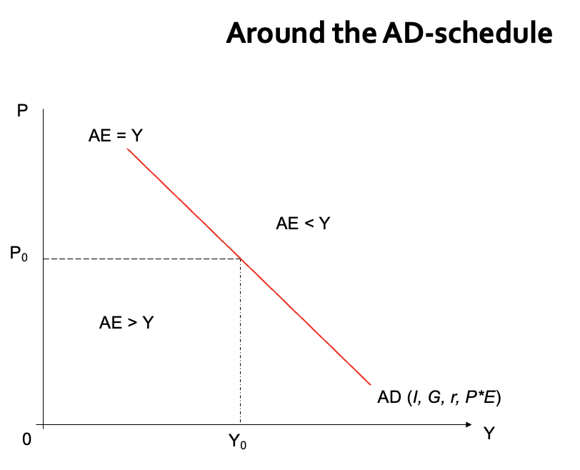
What causes points to lie off the AD curve, and what factors can shift the AD curve?

Points Off the AD Curve:

Left of AD: AE > Y → Upward pressure on GDP as firms can sell more than they produce.

Right of AD: AE < Y → Downward pressure on GDP as firms cannot sell all their production.

Shifts in the AD Curve:

Caused by changes in variables other than price level (P) that shift the AE line, including:

Autonomous consumption (a)

Taxation (t₀)

Net exports (x₀)

Investment (I)

Government spending (G)

Exchange rate/foreign price level (P/E*)

Interest rate (r)

• AE ↑ → AD shifts right

• AE ↓ → AD shifts left

What is the role of the multiplier in determining changes in GDP and the AD curve, and how does it behave when prices rise?

Multiplier Role:

Measures the change in ‘equilibrium’ GDP in response to a change in autonomous spending at a given price level.

On the AD curve, it determines the horizontal shift of the curve when the price level is constant.

• Multiplier Formulas:

  • k = 1 / 1 - b

  • kG = 1 / 1 - b ( 1 - t )

  • ko = 1 / 1 - b ( 1 - t ) + m

    Impact of Rising Prices:

    If prices rise after an increase in AE, the multiplier value is reduced.

    This effect is called supply-side crowding out.

    The degree of reduction depends on how responsive output is to the rise in AE.

• Key Point:

  In this general model, the multiplier depends on both the supply-side and demand-side of the economy.

What is aggregate supply, and how does it relate to production and the AD curve?

Aggregate Supply:

Total output of goods and services that firms wish to produce, assuming they can sell all they wish at the going price level.

Production Process:

Firms use inputs (labour, capital, and raw materials) and transform them into output using technology.

Technology determines the most efficient combination of labour and capital, known as the production function.

Theoretical Issues:

The theory of aggregate supply is abstract and controversial, with unresolved technical challenges.

Simplification:

To align with the AD curve derived so far, it is simplest to think about an aggregate supply relation that avoids these technical issues.

How do firms set prices using a mark-up on average costs, and what happens if labour is the main variable cost?

Pricing with a Mark-Up:

Firms set prices as a mark-up on average prime costs, consistent with firms having some market power.

Empirical evidence supports this behaviour.

• Example:

  • If a microchip costs £10 to produce and the mark-up is 50%, the final price is:
    £10 + ( 0.5 × £10 ) = £15

• General Formula:

  • Pi = ( 1 + μi ) ACi

    • P: Price level of firm i

    • μ: Profit mark-up

    • AC: Average cost

• If Labour is the Main Cost:

  • Average cost equals the money wage rate (W):
    Pi = ( 1 + μi ) Wi

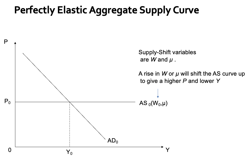
How do we aggregate prices over all firms, and what are the characteristics and limitations of the simple aggregate supply curve?

Aggregation Over Firms:
P = ( 1 + μ ) W
P: Aggregate price level
W: Wage rate
μ: Constant mark-up

Characteristics/Limitations of the Simple Aggregate Supply Curve:
- Prices are driven only by costs → Inflation is always “cost-push.”
- Productivity is assumed constant at all output levels.
- The aggregate supply curve is horizontal in (P, Y) space → No link between output (Y) and price level (P).

Advantage:
This supply schedule aligns with previous assumptions in aggregate demand:
Output is demand-determined.
Price level is supply (cost)-determined.

What are the microeconomic behaviour assumptions we make about firms?

They are profit-maximising, firms operating in a perfectly competitive       environment

This means firms are price –takers in both the output and input markets- so   they have no influence over either P_i or W_i.

Their capital stock  (K) is fixed, and they vary only one factor input , labour (L)

It is assumed that the production function is concave to the origin so that there   is diminishing marginal product of labour (MPL). This means that each extra   worker adds to total output but not by as much as the previous worker.

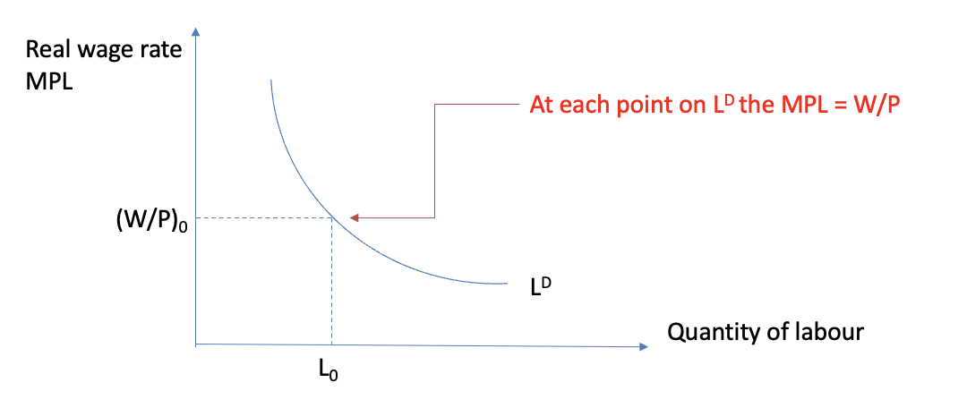
What is the condition for profit maximisation in a firm with respect to marginal cost (MC) and marginal revenue (MR)?

The firm maximizes profit by producing at the point where marginal cost (MC) equals marginal revenue (MR).

• MC is the money wage rate (W), which is the cost of hiring an additional worker.

• MR is the monetary value of the marginal product of labor (MPL), calculated as (ΔY/ΔL) × P = MPL × P.

In equilibrium:

MC = MR or W = MPL or W / P = MPL

If MR > MC, profits are rising, and the firm will increase output.
If MR < MC, profits are falling, and the firm will reduce output and employment.

To maximise profits, the firm sets:

W / P = MPL

What curve do we get after summing horizontally over all firms at every level of wages?

A downwards sloping planned aggregate demand for labour schedule, showing the law of demand. Demand is high at low wage rates, but low at high wage rates.

How can we derive an aggregate supply curve?

An aggregate supply curve (AS) can be derived by asking how planned output varies as the price level changes. 

To show this we assume that the money wage (W) is fixed; that the capital stock (K) is fixed; and that output varies directly with employment in that as more labour is employed more output is produced.

This is displayed in the attached graph.

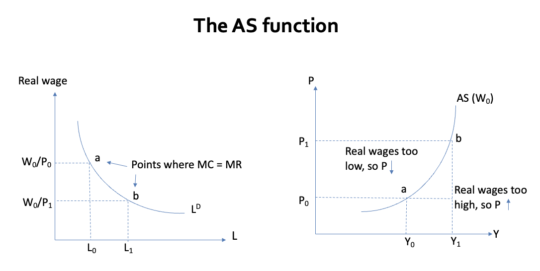
What are the properties of the SRAS relation’s properties?

It has an upwards slope.

It is shifted up (down) by rises (falls) in money wage rates.

Output increases along the curve as the real wage rate falls.

The reason is because as the money (nominal) is held fixed, any change in the price level will change the real value of the wage rate.

This follows because the firm are profit maximisers – with constant cost MC, a rising P implies rising MR and so profits are rising which means firm will continue to produce more output until MC = MR.

This is not good for the workers! As you move along the AS curve to the right the real wage rate falls continually. This is also why this upward sloping curve is sometimes referred to as the short-run curve.

We have derived an upward sloping short-run AS curve – so when combined with the AD curve gives a model of the determination of the price level and output in the short run.

Why don’t Neo-classical economists regard this as a complete story?

We have not fully specified the labour market; we have wholly ignored the supply of labour.

There is no mechanism for the model to gravitate automatically to full employment (capacity) output even in the long run – i.e. we have assumed the need for some policy intervention

What is the distinction between the short-run and long-run Aggregate Supply (AS) curves in economics?

Short-Run Aggregate Supply (SRAS): Shows the quantity of output firms wish to produce, assuming that input prices remain constant (e.g., wages are fixed). This is the case in the short run, as we have been assuming so far.

Long-Run Aggregate Supply (LRAS): Represents the desired quantity of output firms wish to produce after input prices (like wages) have fully adjusted to any demand shocks. It reflects a more flexible, fully-adjusted economy.

Note: The long run, in this context, is different from the microeconomic definition. It refers to the time when all factors of production are variable, and is not directly related to the adjustment of input prices.

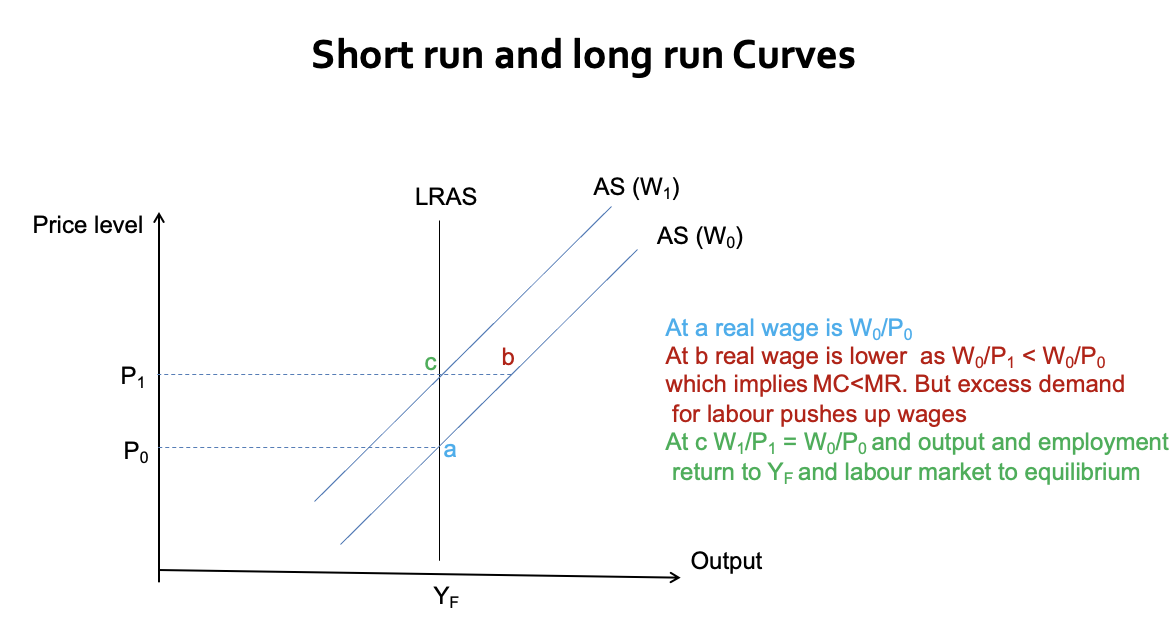
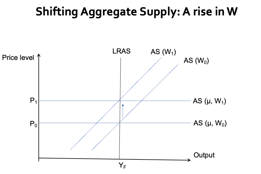
What is the relationship between the real wage rate, equilibrium, and the Aggregate Supply (AS) curve in the short run and long run?

In the short run, the real wage rate (W/P) is changing along the Aggregate Supply (AS) curve, which means there is disequilibrium in the labor market.

Equilibrium (or long-run): In the long run, the real wage rate must be constant to achieve labor market equilibrium (supply equals demand). This happens when the general level of money wages (W) rises exactly in line with the price level (P), so:

ΔW = ΔP

This ensures that the real wage (W/P) remains constant.

Impact on the AS Curve: If wages increase in line with prices, the AS curve becomes vertical at the level of full employment output (YF), also known as potential output (Y)*. This is the market-clearing level of employment, where the labor market is in equilibrium.

What are the key differences between the Keynesian and Neo-classical models regarding the Aggregate Supply (AS) curve and unemployment?

Along the LRAS curve: The real wage rate is constant at all points:

( W / P )0 = ( W / P )1 = ( W / P )2

Short-Run AS Curve: In the short run, the money wage is constant.

• Key Difference:

  • Keynesian Model: Represents a short-run disequilibrium with an upward-sloping AS curve.

  • Neo-Classical Model: Represents an equilibrium with a vertical AS curve at full employment.

• Unemployment:

  • In the Neo-Classical Model, there is no involuntary (demand-deficient) unemployment. All unemployment is voluntary (frictional or structural).

  • The model assumes an automatic return to full employment without the need for government intervention.

How does a rise in labor productivity affect the Aggregate Supply (AS) and Long-Run Aggregate Supply (LRAS) curves?

• Two AS curves are derived:

  • One consistent with involuntary unemployment (where the labor market does not clear).

  • One consistent with no involuntary unemployment, where the labor market is in equilibrium (LRAS).

• Key Assumption: In both models, the demand for labor ensures that MPL = W/P (Marginal Product of Labor equals the real wage).

• A rise in labor productivity increases MPL, which in turn raises the demand for labor and the real wage.

• Shift Factors: Productivity is an additional shift factor for both the AS and LRAS curves.

• Effect of a Productivity Rise:

  • A rise in productivity shifts both AS and LRAS curves to the right.

• Short vs Long Run: A short-run rise in productivity typically affects the LRAS, as it reflects a shift toward the economy’s full potential.

How do competitive labor markets and monopoly power in the goods market affect the AS curve, and what role does productivity and trade unions play?

• Three AS Curves:

  • Two are based on competitive labor markets.

  • One is based on monopoly power in the goods market.

• In competitive labor markets, productivity is an important shift variable, but this is not the case in monopoly markets.

• The idea of an aggregate production function is considered dubious in the monopoly case. The flat AS curve is preferred, with monopolistic or oligopolistic structures.

• Trade Unions: In these models, trade unions can raise the money wage independently of economic factors, shifting the flat AS curve upward to reflect higher production costs.

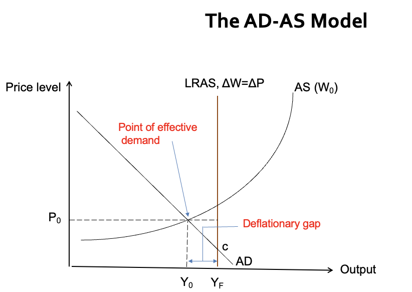
What is the relationship between the AS-AD model, effective demand, full employment, and the concepts of inflationary and deflationary gaps?

• AS-AD Model: The Aggregate Supply (AS) and Aggregate Demand (AD) schedules are combined on the same axes. The point where they intersect is the equilibrium or point of Effective Demand.

• Effective Demand: This point does not necessarily correspond to full employment, but is where suppliers' and buyers' plans are met.

• Full Employment: The point of full employment (or productive capacity) is where demand and supply of labor are equated. However, Keynes did not have a specific labor supply curve, making the concept of full employment ambiguous.

• Labor Supply Constraint: To address this, we assume a labor supply constraint, which defines the maximum output the economy can produce.

• Inflationary Gap: When effective demand exceeds the economy’s maximum output, it creates an inflationary gap: Y0 − YF > 0 leading to inflation.

• Deflationary Gap: When effective demand is less than the maximum output, it creates a deflationary gap: Y0 − YF < 0, leading to underemployment and reduced output.

What is the difference between Keynesian and Neo-Classical views on moving the economy to full employment, and how do they view the role of wages and policy?

• Keynesian View:

  • The economy is stuck at (P₀, Y₀) due to effective demand.

  • There is no automatic mechanism to move the economy to full employment (LRAS).

  • To eliminate an inflationary gap, policy activism is required, not just wage cuts.

• Neo-Classical View:

  • At (P₀), there is an excess supply of output, which should lead to falling prices and money wages, reducing real wages.

  • This would shift the economy to the full employment point (c on the LRAS curve).

• Keynesian Critique:

  • Lowering wages economy-wide would be like cutting aggregate demand, worsening a deflationary gap and deepening the recession.

  • If workers expect future price falls, they may delay spending, sustaining the recession.

• Debate:

  • Keynesians argue that policy action is needed to restore full employment, while Neo-Classicals believe that falling wages and prices will bring about automatic full employment.

What makes the supply-side of the economy difficult to model?

The aggregate production function and the marginal relations are highly   abstract concepts at the microeconomic level: at the macroeconomic level   they are barely implausible

What is appropriate for a firm is not appropriate for the economy as a whole   because of the fallacy of composition. This was ultimately Keynes insight.

The Neo-classical case is interpreted as a long-run equilibrium position which is never reached – but always the objective of policy – while the Keynes short-run story offers a pathways of policy choices to get nearer to the long-run equilibrium, whilst the economy is faced with deflationary or inflationary gaps.

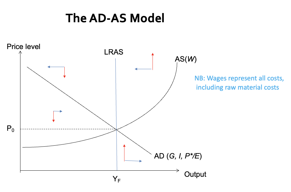
Imagine the AD-AS model and compare how it looks to the real model

What have been the 4 major shocks to the UK economy since the mid 1970s?

The 1970’s oil price shocks 1973/4 and 1979/80

The EMS crisis in 1992

The global financial crash of 2008-9

COVID Crisis in 2019-20

Explain the Oil Price Crisis

• In the early 1970s, the UK relied on cheap oil, mostly imported from the Middle East.

• A war in the region led OPEC to quadruple oil prices in 1973/4 and double them again in 1979/80.

• The demand for oil was inelastic, causing the UK to face a significant rise in production costs and a current account deficit.

• To conserve electricity, the UK implemented a 3-day working week from January to March 1974.

• This crisis represented a large negative aggregate supply shock.

• In the long run, the crisis made the development of North Sea Oil production profitable, and by the end of the decade, the UK became an oil and gas producer.

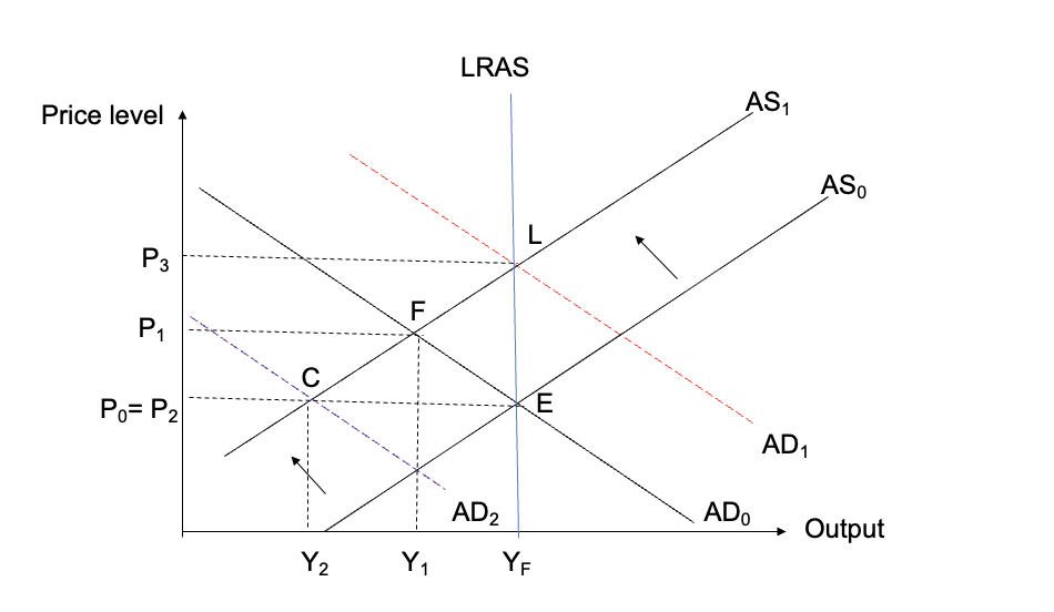
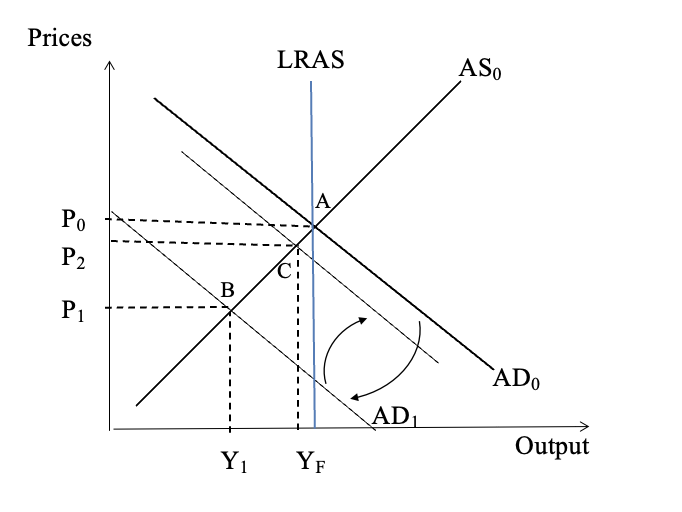
How would an AD-AS model be affected by this? How may you respond to this shock?

From the initial point at E the Oil price rise  shifts AS₀ to AS₁ – giving higher price at P₁ and lower output at Y₁

Option 1: Do nothing wait until unemployment puts downward pressure on money wages and price expectations so AS₁ moves back to AS₀

Option 2: Increase AD to AD₁ to protect employment but take a hit on inflation (Labour Party policy 1974-78) so moving the model from F towards L

Option 3: Cut demand to AD₂ to keep inflation low at all costs and take an even bigger hit on unemployment (Conservative Party policy 1979-83) in response to the second oil shock, so moving from F to a point like C.

Explain the EMS shock

• In September 1990, John Major, the successor to Mrs. Thatcher, decided to join the EU's fixed exchange rate mechanism (ERM) to demonstrate pro-European credentials.

• The UK joined the ERM at an overvalued exchange rate (10-14% overvalued), leading to a recession and a self-inflicted negative aggregate demand shock.

• The overvaluation caused high unemployment.

• The UK exited the ERM in September 1992, and the pound was devalued by about 14%, which restored demand.

• This marked the start of the 'great moderation' (1992-2009) until the next financial crisis.

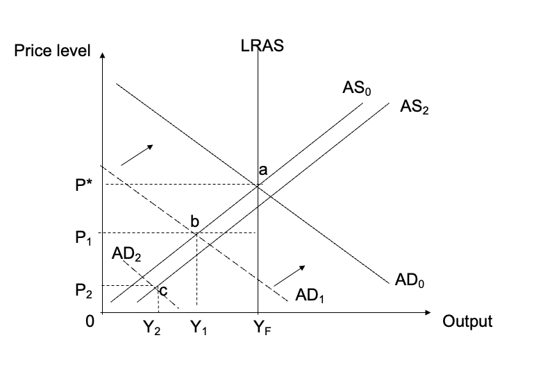
How would an AD-AS model be affected by this? How may you respond to this shock?

A large negative demand shock – shifting AD₀ back to AD₁

Option 1: Take a hit on unemployment and wait until in the long run wage and price expectations adjust downwards – restoring output back to its equilibrium level (John Major’s Conservative Party policy 1990-92) Model moves from A to B with lower output and price level.

Option 2: Admit policy mistake and devalue £ against other EMS currencies, hence shifting the model from B back towards C.

Option 3: Wait for a speculative attack to destroy the credibility of the fixed rate policy, forcing the £ out of the system and bring about a 14% devaluation of the £ and shift AD curve back to the right towards point C (which is what happened in September 1992).

Explain the global financial crash of 2009

• The Great Moderation (1992-2008) was driven by:

  • Inflation target setting

  • Central bank independence

  • Extensive international financial integration through liberalisation and deregulation.

• Deregulation led to the rise of syndicated loans and the marketing of mortgages.

• The collapse of US house prices in 2006-07 caused sub-prime borrowers to default on loans, leading to the insolvency or illiquidity of commercial banks.

• To prevent the collapse of banks and the international financial system, the Bank of England and Federal Reserve injected billions into the system and nationalised some banks.

• This led to a lack of credit and collapsed investment, resulting in a large negative demand shock.

How would an AD-AS model be affected by this? How may you respond to this shock?

Effectively a large negative demand shock – shifting AD₀ to AD₁ and the model from a to b.

Option 1: Nationalise or bail out private banks – bankrupting governments, but maintaining the payments system. Cut AD further, to say AD₂, taking the equilibrium to point c, because of excessive public deficits and debt (ECB policy 2008-2013)

Option 2: Bail out banks, but use special measures (quantitative easing) to try to repair banks’ balance sheets so reducing the need for public sector cuts (UK and US policy 2008-15), so moving the model from b back towards a.

Option 3: As option 2 but with a fiscal deficit enlargement to protect employment and actively stimulate economic growth (Nobel prize winners – Krugman and Stiglitz). Deemed to be too risky.

Explain the COVID-19 shock on the economy

• The COVID-19 pandemic caused an unprecedented supply shock by directly impacting labor supply, as serious illness prevented people from working.

• The subsequent lockdown led to a year-long period of limited labor supply, representing a huge negative supply shock.

• Unlike previous shocks (e.g., oil crises of the 1970s), this was a shock to the quantity of labor, not just the price, making it more difficult to alleviate.

• Incomes collapsed due to lack of work, leading to a decline in demand.

• This crisis involved an inflationary supply-side shock and a contractionary demand-side response.

• The pandemic caused unprecedented damage to the economy, comparable to the effects of World War II.

• There was significant uncertainty about the duration of the crisis, death tolls, and how to address the resulting economic problems.

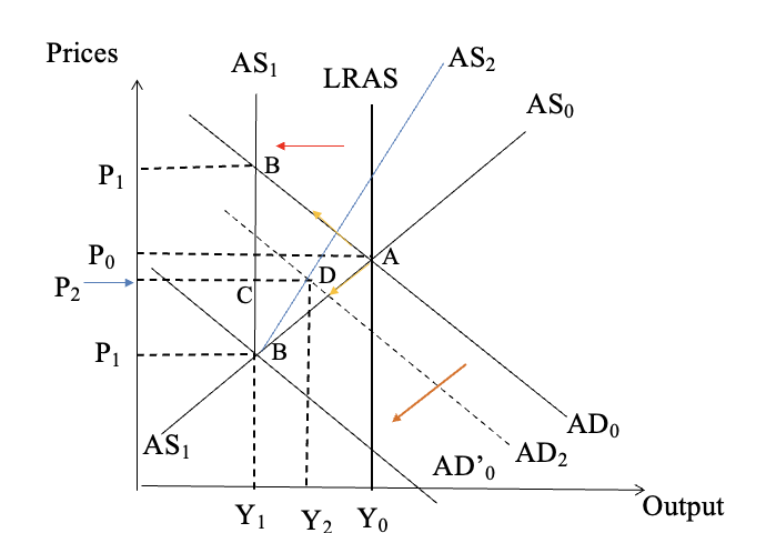
How would an AD-AS model be affected by this? How may you respond to this shock?

Huge negative supply shock which had a direct effect on aggregate supply and demand. Starting from A  the model suggests a movement to B – which B depends on the strength of the open economy effect. As exports collapsed and imports rose – AD falls to AD’₀  and the initial inflationary surge expected doesn’t materialise.

Option 1:  No lock down to get AS moving to the right asap. Problem if working age people perish the LRAS curve will be shift to left permanently reducing capacity. Not really an option ! Moreover, lack of workers likely to push up wages moving AS to the left rather to the right.

Option 2: To try to maintain personal incomes although people not working – the furlough scheme; this supports demand so move from B to C. As lockdown eases AS curve flattens, and we move to point D. Any permanent damage to supply capacity means LRAS will be moving left and a return to Y₀ will not happen for some time.

Long run consequence – massive government borrowing by western democracies to save lives – further endangers the still fragile financial system. Western economics are very much poorer, living well beyond their means -  making current levels of welfare support are unsustainable. Which is a very serious problem for the liberal democracies.

What is the impact of government policies on aggregate demand and supply-side of the economy?

• Government policies can influence aggregate demand through fiscal and monetary policies (e.g., interest rate changes), but have little direct impact on the supply-side of the economy.

• Since the 1970s oil price crises, governments have tried supply-side policies to stabilize and grow the economy, but they’ve only been successful in the short term.

• Incomes policies (e.g., 1975-79) were effective in reducing inflation but were deemed unfair, unsustainable, and against the ethos of a competitive labor market.

• Evidence is weak that cutting supply taxes (like national insurance contributions) stimulates effort, and reversing tax cuts may harm work effort.

• Labour training schemes have had some success, but many are inefficient and offer training in unwanted skills.