PSYC3290 FINAL!!!!!

**What is Standard Error of the Mean (SEOM):

it is the standard deviation of the sampling distribution of the sample mean (MEAN HEAP) that tells us how precise our estimate of the population mean is (measure of sampling variability)

How do you calculate SEOM with a true population SD?

SEM = pop SD/sqrt N

When the sample size increases, what happens to the standard error of the mean?

a) It decreases

b) It increases

c) It remains constant

d) It fluctuates randomly

a) it decreases

How do you calculate SEOM without the true population SD?

take the sample standard deviation (s) instead of the population standard deviation and divide by the square root of the sample size

**What is the central Limit Theorem:

states that the sum, or the mean, of a number of independent variables has, approximately, a normal distribution, almost whatever the distributions of those variables larger N, closer the distribution of T and curve is to normal. (distributions produce a roughly normal sampling distribution of sample means)

Which of the following is a correct implication of the Central Limit Theorem for hypothesis testing?
a) It allows us to use the normal distribution when the sample size is large enough, even if the population distribution is not normal
b) It requires that the population distribution is always normal
c) It only applies to studies with small sample sizes
d) It invalidates the use of t-tests for large samples

a) It allows us to use the normal distribution when the sample size is large enough, even if the population distribution is not normal

According to the Central Limit Theorem, what happens as the sample size increases?
a) The sample means become less variable
b) The sample means become more variable
c) The sample means tend to form a uniform distribution
d) The sample means become identical to the population mean

a) The sample means become less variable (and approach a normal distribution! - large sample size means more ability to infer population characteristics from sample)

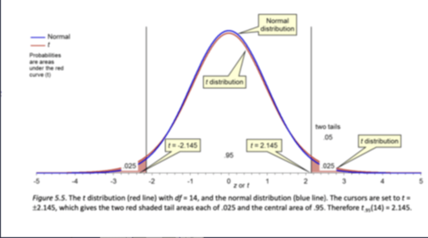
**what is the t-distribution:

very similar to normal distribution but with HIGHER TAILS, we cant use 1.96 anymore and here we have 2.145 as our new limits for 95% CI, this is bc not only does our estimate of µ vary from sample to sample, but our estimate of σ does too!(The larger the df (sample) the closer to the normal distribution your t distribution will be)

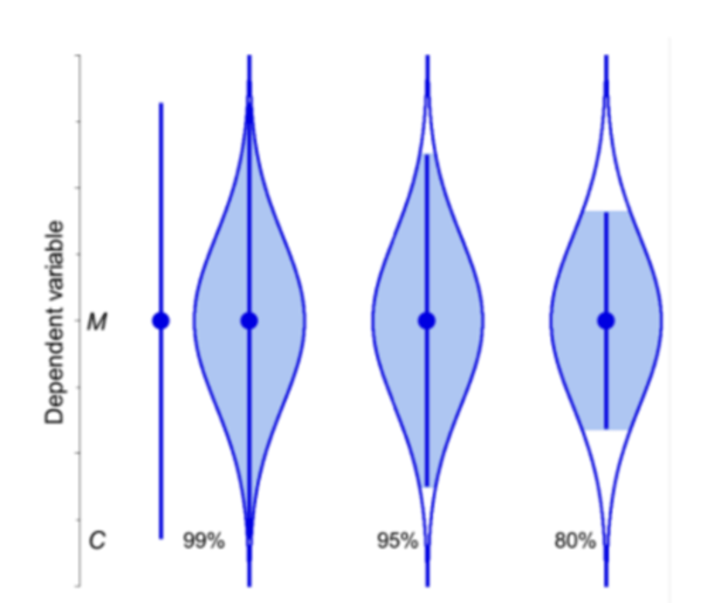
cats eye picture tells us:

how to interpret CI, says not all values in the range are likely to be population, if they are in the middle they are more likely than on outside! as you move away from it, it becomes less likely to true mean

(a CI has C% likelihood of capturing µ, graphically illustrated in a cats eye)

what does the t distribution represent:

the probability of different outcomes for a sample mean when the true population mean is unknown! (especially for SMALL sample sizes)

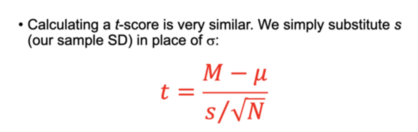
how do you calculate a t-score?

T = M-µ / s /√N (sample mean-population mean divided by sample standard deviation / square root of N)

**What is power:

the chance of CORRECTLY REJECTING the null hypothesis if it is in fact FALSE (corresponds to beta 1 - β - the probability that we can detect said effect and reject the null)

what is power influenced by?

1) alpha (larger alpha = greater power needed to detect an effect, increases type I error)
2) Effect size (larger effect = greater power to detect it)
3) sample size (N)

What does a power of .08 represent?

the likelihood that a study will correctly reject the null if the alternative hypothesis is true. 80% chance of avoiding Type II error!

** What is sampling variability:

the variability in results caused by using different samples (if you repeatedly take samples of the sample size from a population and calculate the mean of each sample, the means will differ!)

post hoc analysis:

(after the fact) is not specified in advance. It risks merely telling us about sampling variability, but may provide valuable hints for further investigation

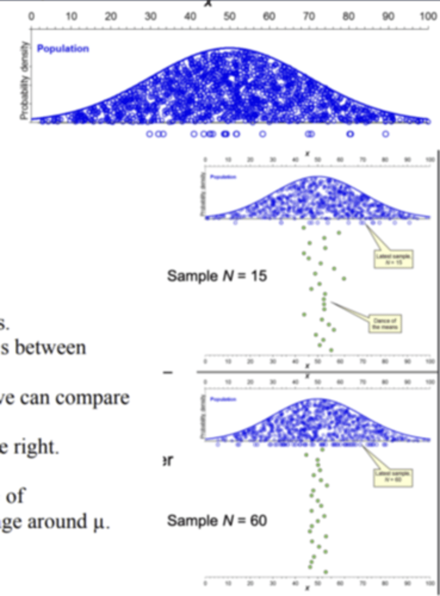
**What is the dance of the means:

sampling variability creates the visual effect of the means dancing around the population mean (Distribution created by the means of many samples the little dots below the X value are the sample Green dots = sample means)

**What is Type I Error:

Rejecting the null hypothesis when its true (false positive)

**What is Type II Error:

Failing to reject the null hypothesis when its false (false negative)

Independent group design has the ability to:

estimate the p-values based on OVERLAP of CIs (utilizes a p value, graph overlap - inter-individual variability)

Paired design has the ability to:

have a no overlap rule (intra-individual variability)

crtitical t vs obtained t value is:

what you get using a table that tells us which t values contain 95% of the scores middle VS. a t value you get from a calculated sample

**Gap between CIs (Independent groups):

the p-value is less than .01 (significant)

just touching CIs (independent groups):

the p value is -.01 (significant)

moderate overlapping CIs

the p value is -.05 (insiginificant)

large overlapping CIs

the p value is greater than .05 (insignificant)

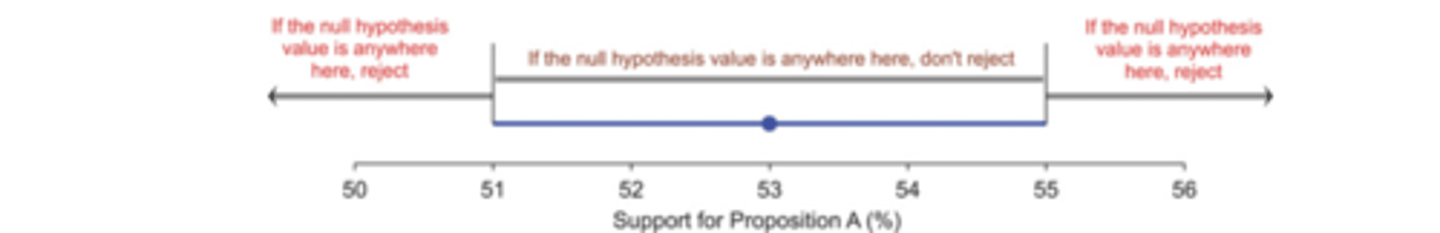
we use CI to evaluate the null by:

comparing the null hypothesis value to the CI (If the hypothesized value falls within the interval, we fail to reject the null hypothesis. If the hypothesized value falls outside the interval, we reject the null hypothesis)

**What is cohen's D:

a standardized effect size measure which is expressure in standard deviation units (assesses the standardized difference between two means in terms of standard deviation)

how to calculate cohen's d:

d = effect size in original units / appropriate standard deviation (ES/SD) for independent groups : d = (M1 - M2) / sp

how to interpret cohen's d:

small = .20
medium = .50
large = .80

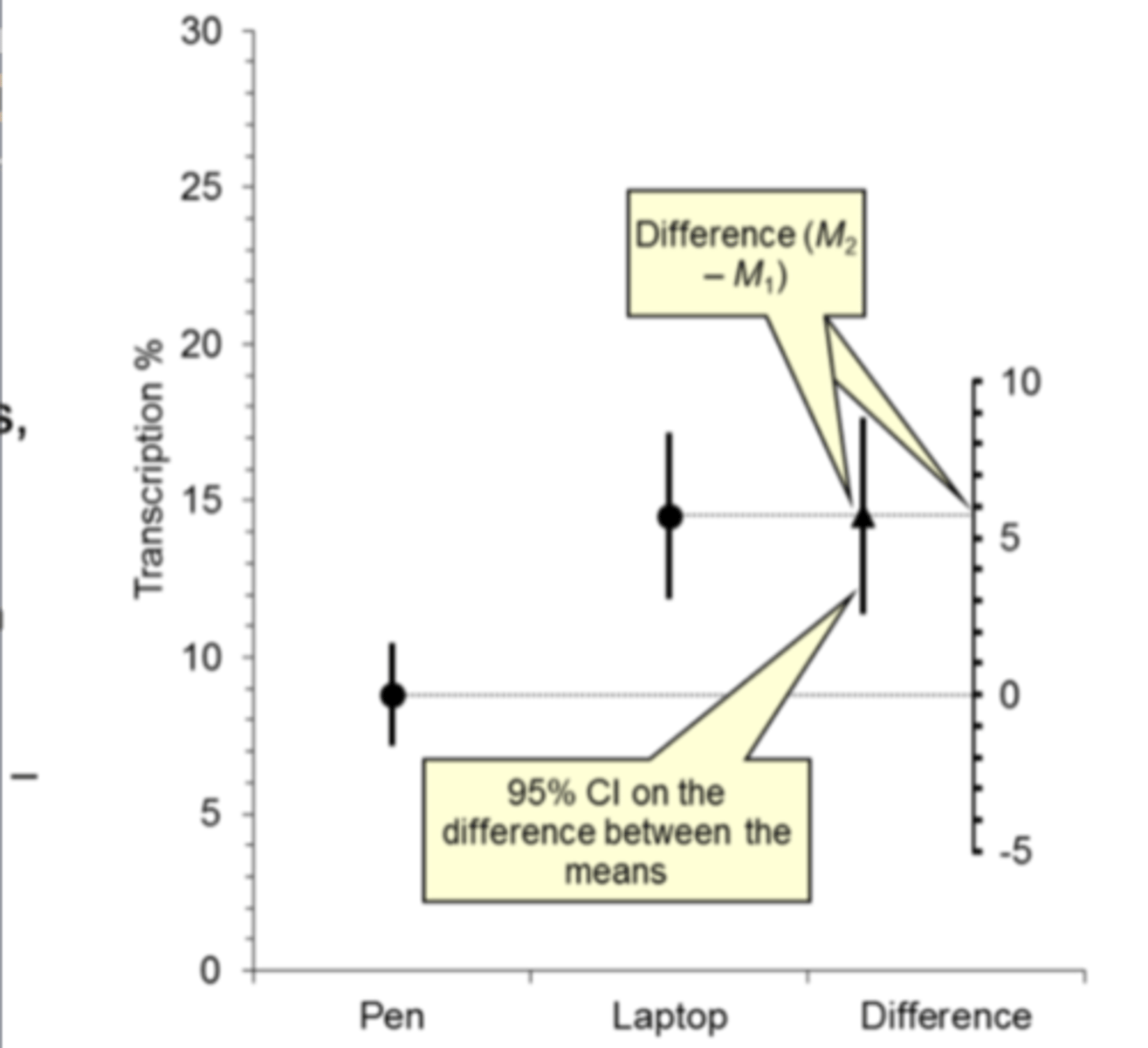
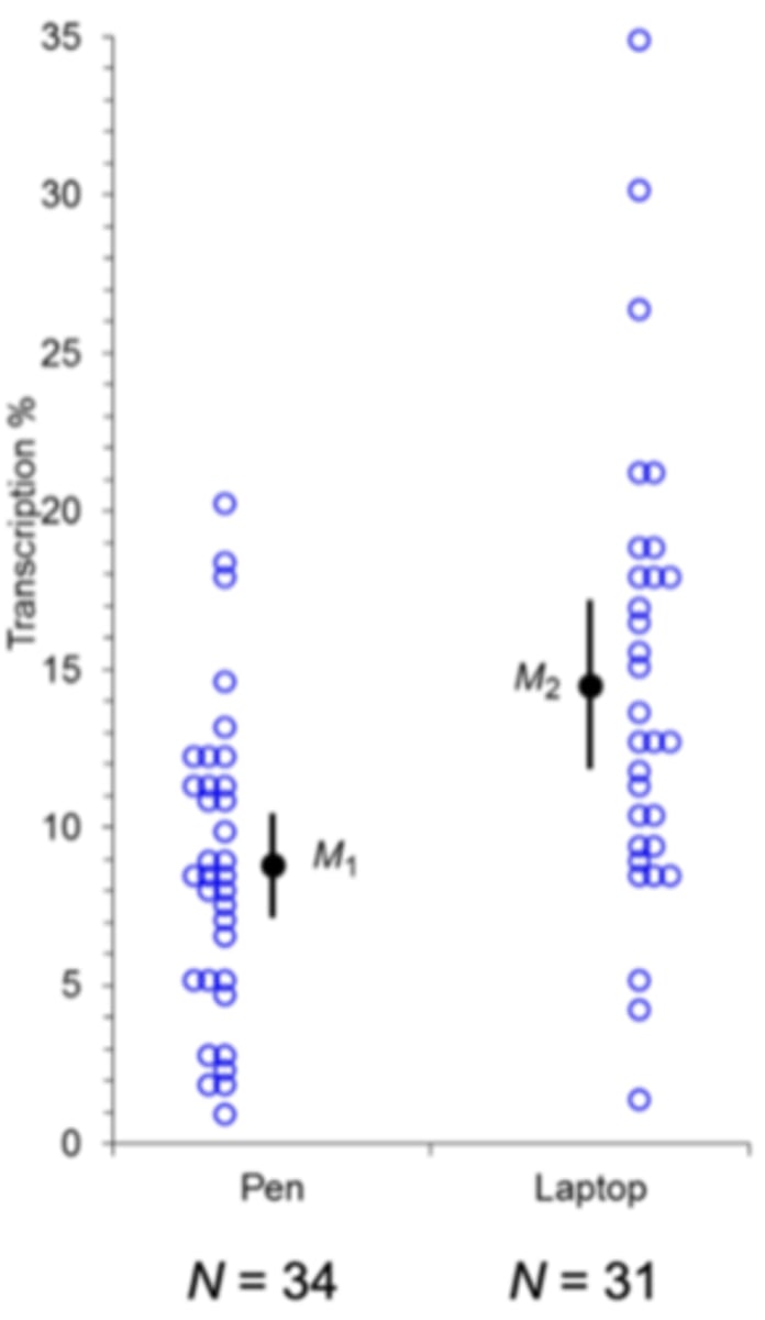
**CI on the difference between 2 means is:

the difference between the 2 group means (m2-m1) (either laptop or pen group, here the difference is 0 which means it is not a very likely mean difference, so we reject the null hypothesis)

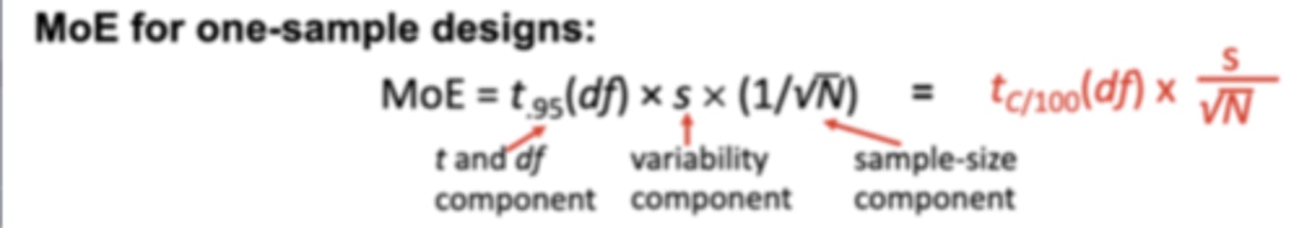
MOE for one sample design calculation:

MOE = t.95 (df) X s (1/sqrtN)

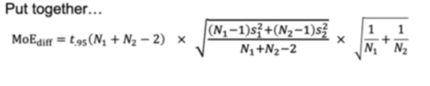
MOE for CI difference calculation (for more than one sample design):

MOEdiff = t.95 (N1 + N2 - 2) X ...

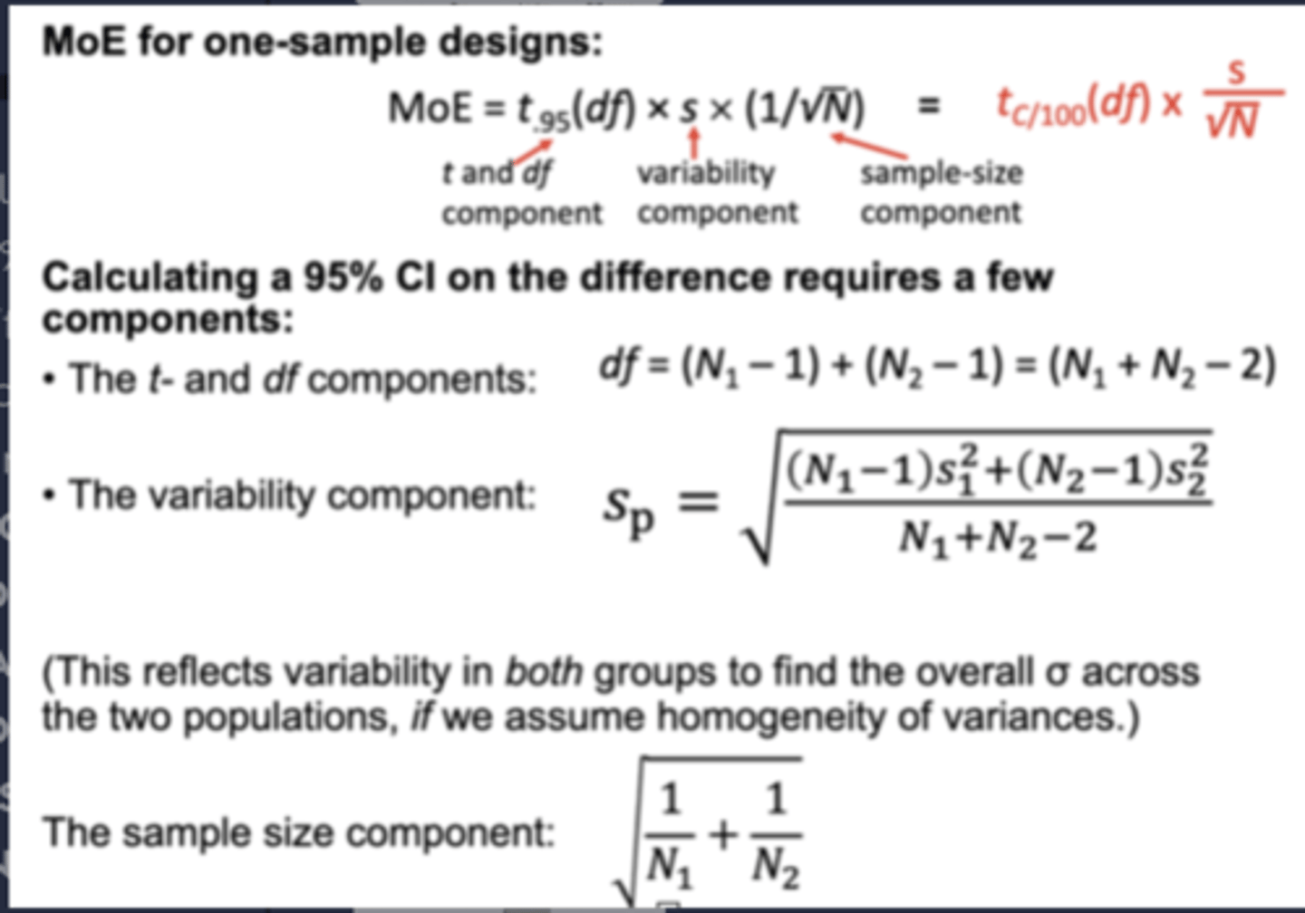
Calculating the 95% CI on the difference requires a few components which are:

1) the t- and df component
2) the variability component
3) the sample size component(use critical t to calculate MoE)

**What is true about sample size:

1) generally, the larger the better (4x the sample size cuts the CI by HALF)
2) when sample size is larger, mean heap is narrow
3) larger the sample, lower the odds of Type II error
4) larger the sample, more likely to detect an effect if it stil exists

small sample size means:

wider distribution of sample means(less precise, longer CI, and bigger MOE)

larger sample size means:

narrower distribution of sample means (more precise, shorter CI, and smaller MOE)

if you have a narrow confidence interval around population mean estimate you will have _______ precision in your estimate

high

what is a paired design?

IV is a within groups variable/repeated measure (all participants experience same conditions) pretest and postest)(compares the means of two measurements taken from the same individual, object, or related units)

- recommended when sample sizes are SMALL

- participants are given a more precise CI on difference than either CI for the means

- no overlap rule is possible

EX: depressed people going to therapy before vs after

What is an independent groups design?

between groups variable, utilizes different participants are used in each condition of the IV

- recommended for LARGE samples

EX: pen vs laptop group

**scenario question 1 EX- figure out the type of design being used: A researcher is running a study looking at the effects of epidural dosages and time on patients’ comfortability while in labour. Patients received only one of three epidural dosages (dose A, dose B, dose C) and are measured at two time-points (10-minutes and 20-minutes).

Split plot ANOVA

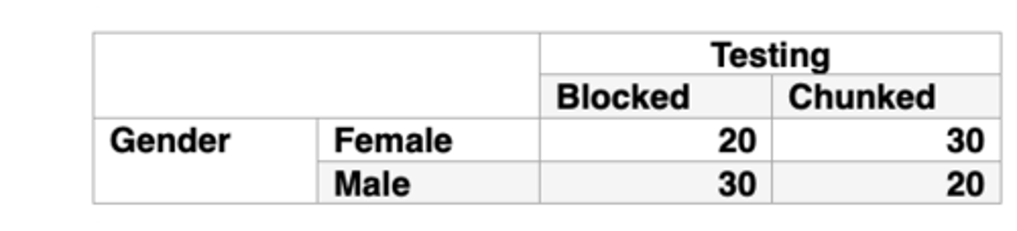
**scenario question 2 EX- figure out the type of design being used:

Interaction between testing and gender

**scenario question 3 EX- figure out the type of design being used: A researcher is trying to decide one which design best fits her research study. She’s looking at the effects of exercise on anxiety levels. Her exercise conditions include running, walking, jumping rope, and weights, such that every participant completes every condition

Repeated measures One-Way ANOVA

**scenario question 4 EX- figure out the type of design being used: A researcher is running a study looking at the effects of epidural dosages and time on patients’ comfortability while in labour. Patients received only one of three epidural dosages (dose A, dose B, dose C) and are measured at two time-points (10-minutes and 20-minutes).

a. How many hypotheses will the researcher be testing with this design?

Three

**Scenario question 5 EX- figure out the type of design being used: A researcher is studying the effects of two different teaching methods (traditional vs. interactive) on students' test scores. The researcher also wants to examine whether the effect of teaching method depends on students' prior knowledge level (high vs. low).Each student is assigned to one of the teaching methods based on their prior knowledge, and their test scores are measured at the end of the study.

Factorial ANOVA (between subjects) (explanation: there are 2 IV's both IVs are between-subjects factors, DV is test scores

**Scenario question 5 EX- figure out the type of design being used: A researcher is studying the effects of teaching method (lecture-based, discussion-based) and assessment type (written exam, oral presentation) on student performance. Each student is randomly assigned to one teaching method and completes both assessment types.

Split Plot ANOVA (explanation: there is one between group IV which is teaching method and students are each assigned to a group, and one within-subjects IV which is assessment type, where each student experienced BOTH levels)

**Scenario question 5 EX- figure out the type of design being used: A researcher is studying the effects of teaching method (lecture-based, discussion-based) and assessment type (written exam, oral presentation) on student performance. Each student is randomly assigned to one teaching method and completes both assessment types.

a) How many independent variables are in the design?

two (teaching method (between) and assessment type (within)

**Scenario question 5 EX- figure out the type of design being used: A researcher is studying the effects of teaching method (lecture-based, discussion-based) and assessment type (written exam, oral presentation) on student performance. Each student is randomly assigned to one teaching method and completes both assessment types.

b) if a significant interaction effect is found between teaching method and assessment type, what does this mean?

the effect of teaching method depends on the type of assessment

**Scenario question 5 EX- figure out the type of design being used: A researcher is studying the effects of teaching method (lecture-based, discussion-based) and assessment type (written exam, oral presentation) on student performance. Each student is randomly assigned to one teaching method and completes both assessment types.

c) if the main effect of the teaching method is significant, what conclusion can the researcher draw?

one teaching method outperforms the other across all assessment types

**Scenario question 5 EX- figure out the type of design being used: A researcher is studying the effects of teaching method (lecture-based, discussion-based) and assessment type (written exam, oral presentation) on student performance. Each student is randomly assigned to one teaching method and completes both assessment types.

d) If the researcher finds significant differences in student performance and wants to determine which teaching method or assessment type is driving the results, what type of post hoc test should be conducted?

Bonferroni correction

what is a bonferroni correction

used in within-subject comparisons to adjust for multiple comparisons

What is a tukey HSD:

suitable for post hoc test of between-subjects factors when theres multiple groups

How to determine if its a factorial or One-way ANOVA

factorial ANOVAs: has one or more independent variables one-way ANOVA: always has only one dependent variable

**What is Sum of Squares:

a way to measure how spread out a set of data points are from the mean, the sum of the squared differences between each data point and the mean (In a One-Way ANOVA each variability term is calculated using the sum of squares (SS)

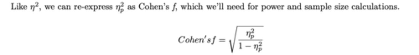
**In a factorial II ANOVA you can calculate for cohen's f using N2p and the two IV's SS's:

f = √n2p/ 1-n2p

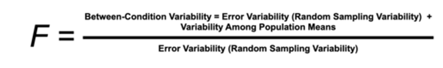
**in the case of a one-way between subjects ANOVA, you need the f distribution which is calculated as:

f = between group variability + error variability + variability among population means / error variability

when you run a factorial anova and your testing 3 null hypotheses at the same time what are looking for:

1) main effect of IVa
2) main effect of IVb
3) interaction between A and B
(null is that there is no effect of Iv1 and no effect of IV2, and interaction)

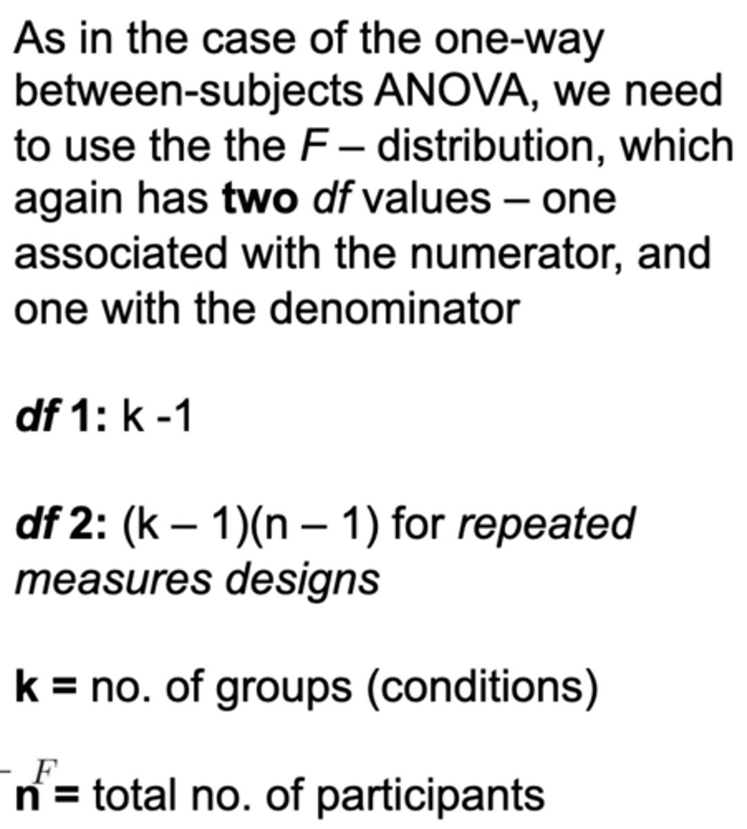
what do the 2 df values in one-way ANOVAs represent?

df 1 : k-1
df 2 : (k-1) (n-1) (repeated/within measures design)

k = number of groups

n = total number of participants

Obtaining SStotal means:

includes the variability associated with SSIV 2 and the interaction between IV1 and IV2 SSIV 1∗IV 2 (when more than one IV is present, η 2 p will always be larger than η 2 )

**What is the appropriate effect size measure for a one-way ANOVA repeated measures within or between?

eta-squared, or partial eta squared n2 (n2 = SSeffect/SStotal) shown as a percentage

**what is the appropriate effect size measure for factorial and Split plot ANOVAs (factorial within or factorial between)?

partial eta-squared, η 2 p (n2p = SSIV/ SSIV + SSerror)

Effect size for T tests:

cohen's D

effect size for correlations:

r2 (percentage)

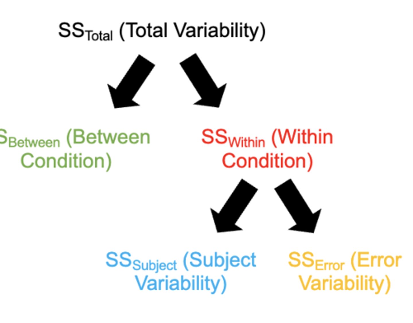
what do sums of squares generally represent:

it measure the total variability in the data, into between-group and within-group variability

How are sum of squares used in calculation of f statistic?

this specific statistic compares the variability explained by the model SS between tp the unexplained variability using the formula: F=MS(mean square) between/MSwithin

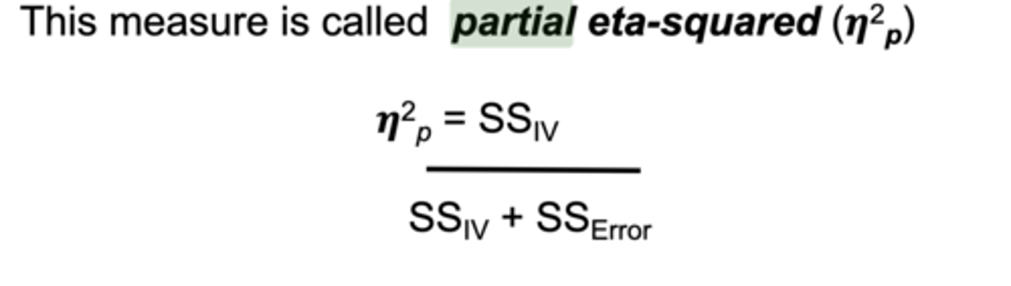
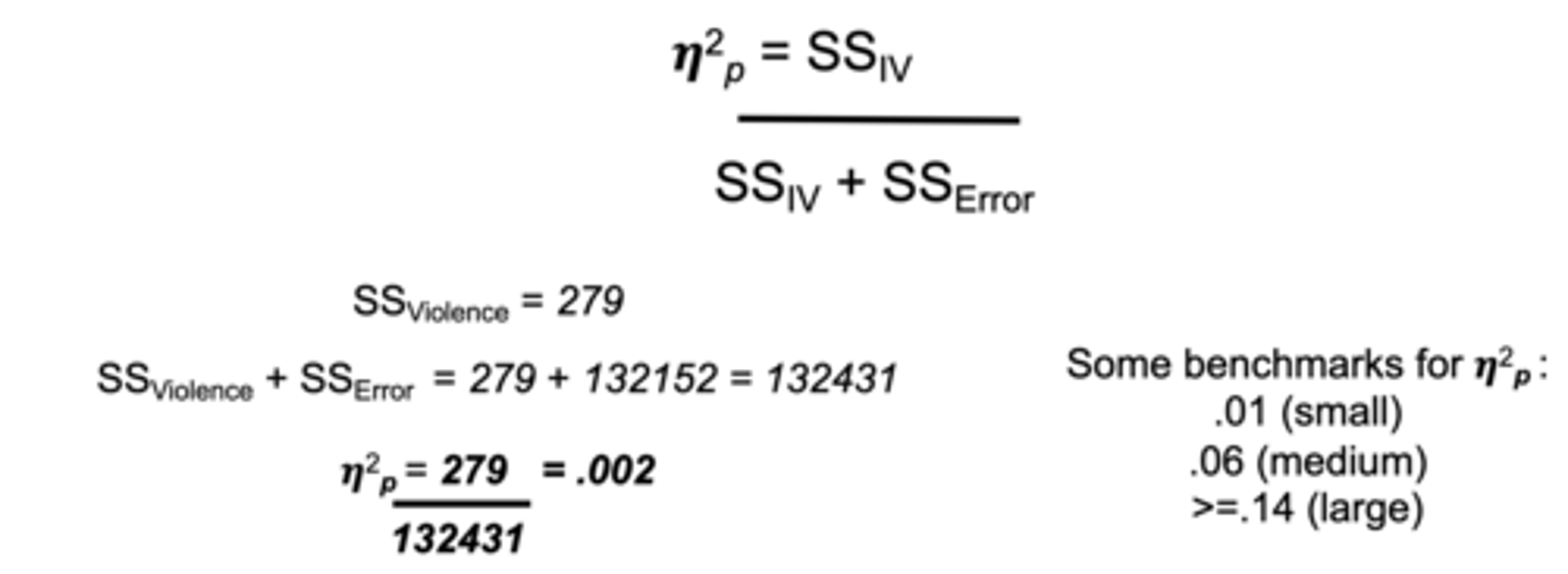
**What is partial eta-squared (𝜼 2p):

(more than one independent variable) An effect size estimate which can be computed for each main effect and interaction. Each of these effect size measures expresses SSIV as a proportion of SSIV + SSError

Some benchmarks for 𝜼 2p:

.01 (small)

.06 (medium)

>=.14 (large)

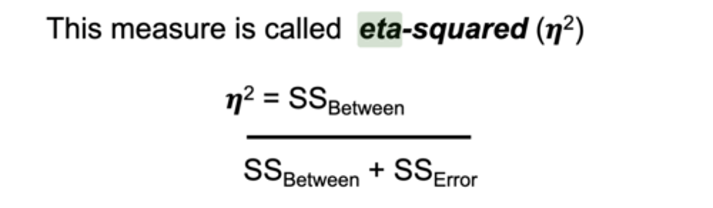
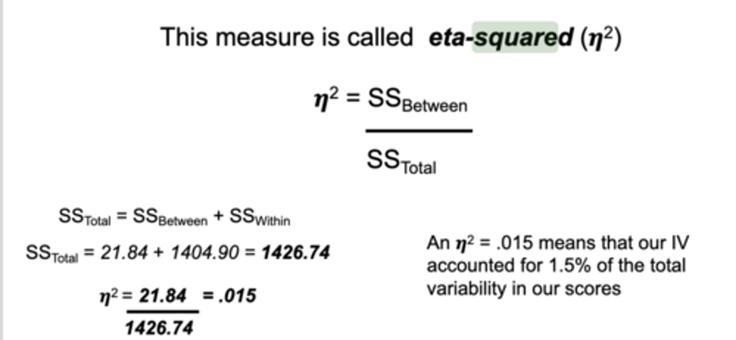
**what is eta-squared (n2)?

(one independent variable) name of the measure of a one-way ANOVA effect size (measured by expressing the between-groups variability (SSBetween) as a proportion of the total variability (SSTotal))

Some benchmarks for 𝜼 2:

.01 (small)

.06 (medium)

>=.14 (large)

Sphericity Assumption is:

The variability of the difference scores between each pair of conditions must be equal

**basic relation between a 95% CI and the p value is stated as:

- if the null hypothesis value lies outside of the 95% CI, the p value is less than .05, so p is less than the significance level and we reject the null hypothesis
- if the null hypothesis lies inside the 95% CI, the p value is greater than .05, so we dont reject

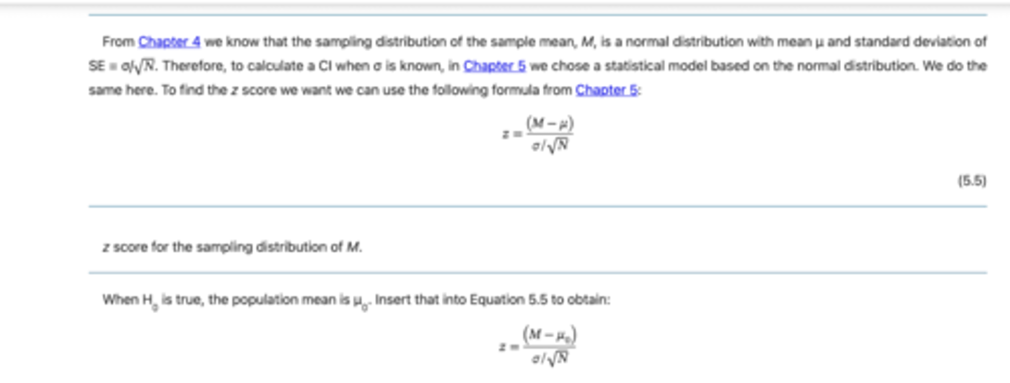
z score formula (FOR KNOWLEDGE):

Z = (M - µ) / alpha/ sqrt N)

**Correlation r is:

measure of the strength of association between 2 variables, such as ratings from -1 through 0 to +1

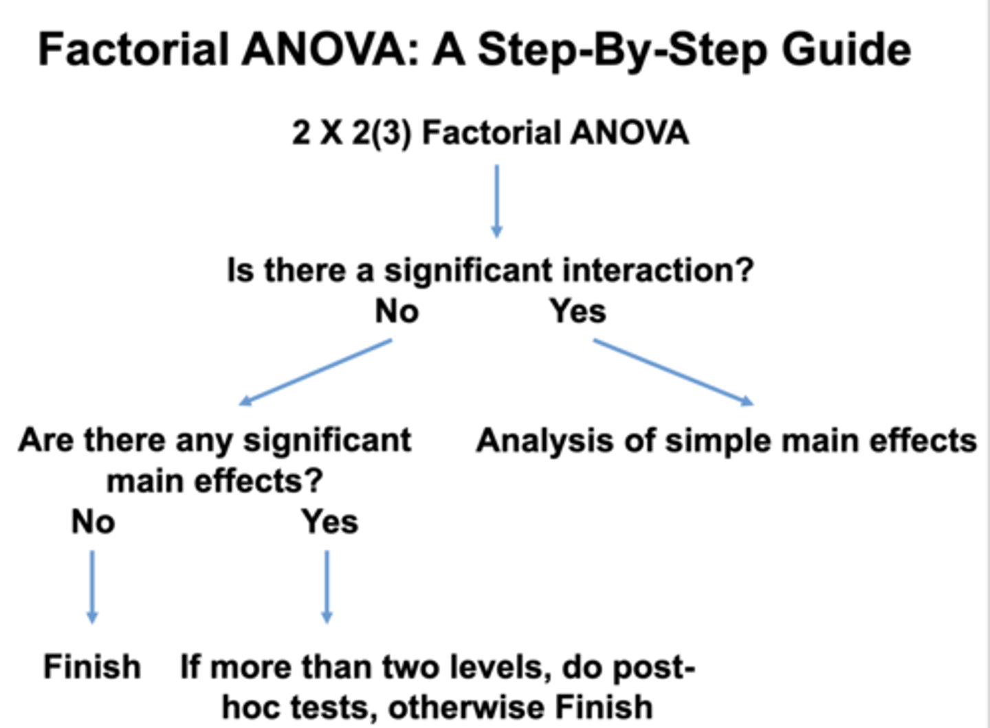
factorial anova guide if there is an interaction:

analyze the simple main effects

factorial anova guide if there is NOT an interaction:

if there are no simple main effects your finished... BUT if there is between 2+ levels complete a POSTHOC TEST

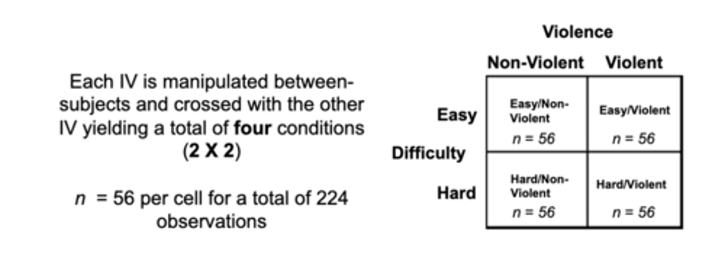
**designs with more than one IV design (factorial 2 X 2) looks like:

chart has 2 IVS: violence and difficulty with 2 levels : easy and hard

**What is between variability:

seeing the difference between each group mean to overall mean (reflects the variability caused by IV) (AKA control, white, music)

**What is within variability:

seeing the difference within each group's data points in comparison each group mean, reflects the variability due to random factors NOT IV (participants)

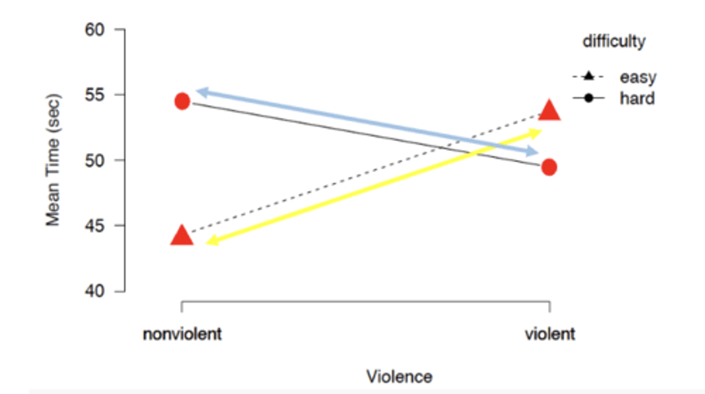
**What is simple main effect?

when there is an interaction, determines where the difference lies in an interaction by comparing the effect of IV1 at each level of IV2, or conversely, the effect of IV2 at each level of IV1

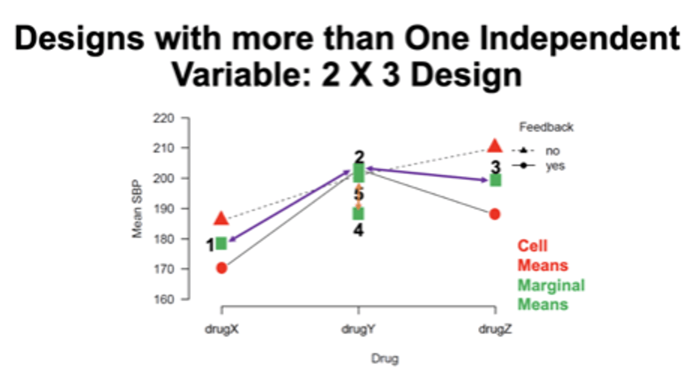
EXAMPLE: difference between red triangle and another red triangle

what does a significant interaction mean?

that the effect of one IV depends on the level of the other IV (existence of NON parallel lines)

EXAMPLE: comparing 3 circles or 3 triangles, (if one isnt and other are just test for significant one!)

**when is it appropriate to analyze main effects?

when theres no interaction, focusing one one IV and you found one IV is significant

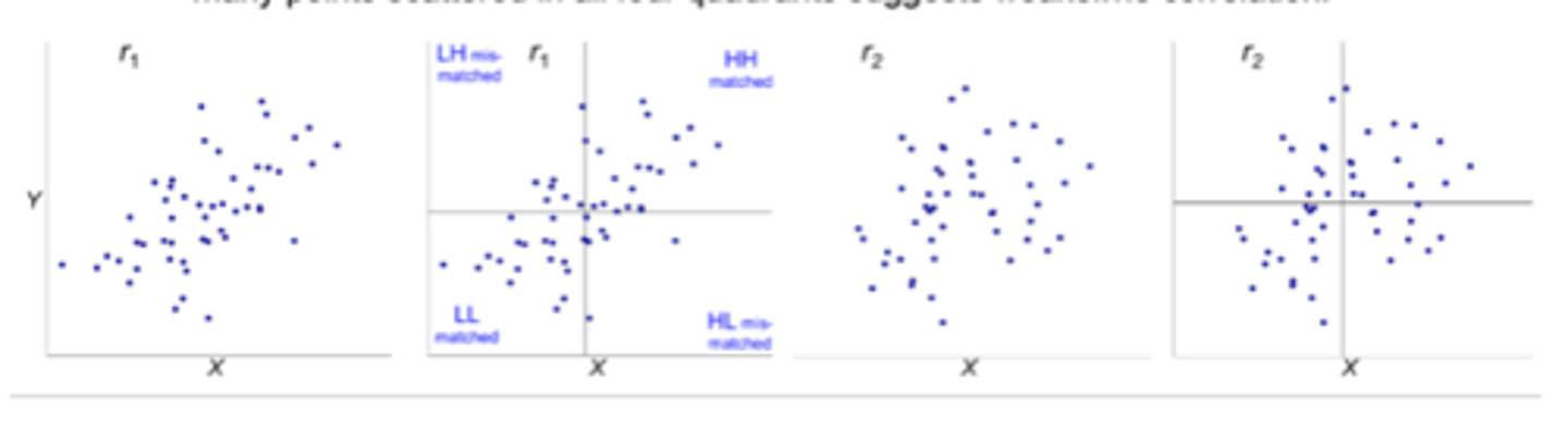
what is the difference between r = .1 and .9 on a scatterplot??

the strength and pattern of the relationship between the variables X and Y:

Correlation r=.1

Strength: Very weak correlation.

Scatterplot Appearance: The data points will be widely scattered with no clear trend. There’s only a slight tendency for Y to increase (or decrease) as X increases.

Interpretation: A small positive correlation indicates a weak linear relationship. Knowing X gives very little predictive power about Y

Correlation r=0.9

Strength: Very strong positive correlation.

Scatterplot Appearance: The data points will be tightly clustered along a straight line sloping upwards. There’s a clear pattern showing that as X increases, Y also increases in a predictable way.

Interpretation: A large positive correlation means a strong linear relationship. Knowing X provides high predictive power about Y

**how to identify if a scatterplot is showing a negative or positive correlation?

more matched = positive correlation

EX: more sleep hrs are associated with better cognitive test scores

(both variables move in same direction (as one increases so does other)

more mismatched = negative correlation

EX: fewer sleep hrs correlate with lower cognitive scores

(variables move in opposite directions, as one increases other decreases)

(NO RELATION: sleep hrs and cognitive performance are unrelated)

**Dance of r values is measured by:

correlation coefficient

r = +1 perfect positive relationship

r = -1 perfect negative relationship

r = 0 no relationship

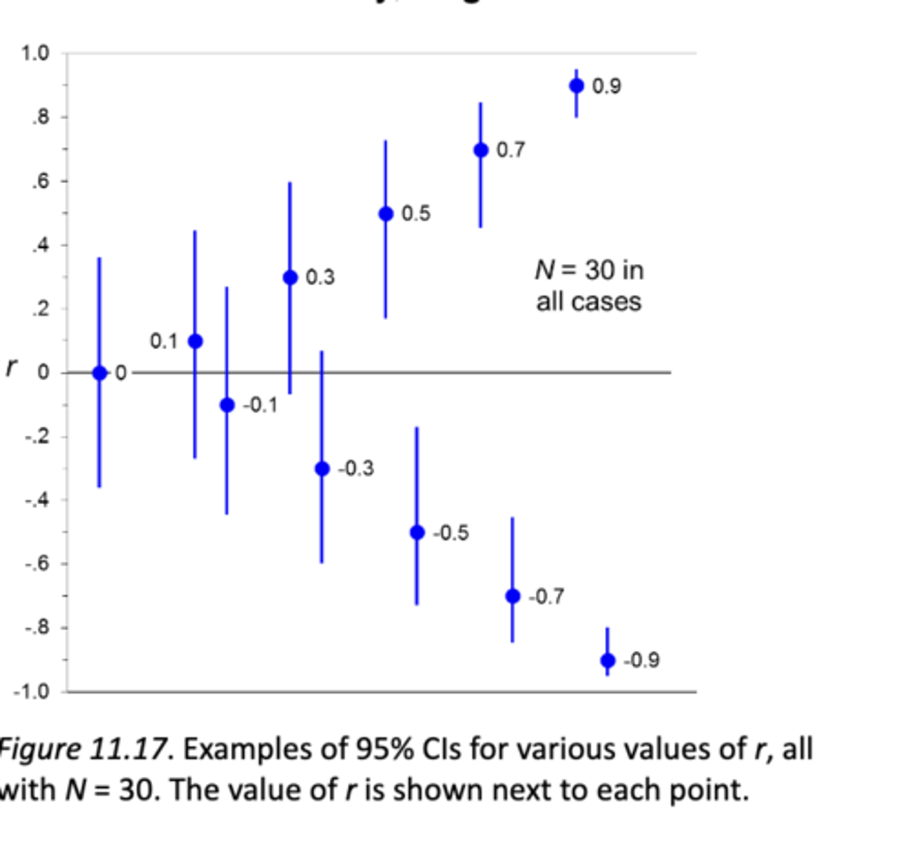
**Confidence Intervals around Pearson's r:

r can be used to estimate ρ. r values dance for smaller Ns!!

(if CI overlaps 0 = possible fail to reject null as 0 is possible if its in range)

(the lower the value the more confident you are that true pop is .5 null = 0)

how does this scatterplot showing the 95% CI for r show asymmetry of CIs on r:

r = 0; long and symmetric CI—as r gets further from 0, the CI gets shorter andmore asymmetric, with the side further from 0 as the smaller side.

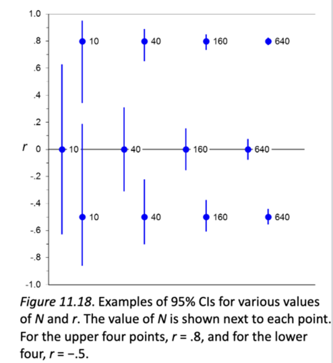
how does this scatterplot showing the 95% CI for r show an effect of N on CIs on r:

Predictably, larger N results in a shorter CI

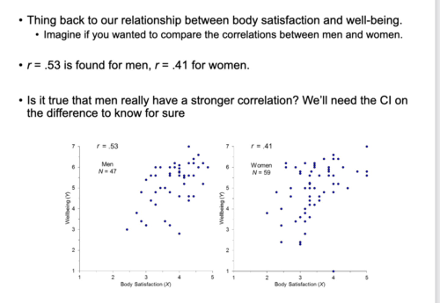
the CI on the difference of r allows us to:

tell the difference if one variable has a stronger correlation than another variable

**Line of best fit is calculated by:

finding the line that minimizes the squared differences between actual data points + predicted values on line. Ensures the best representation of relationship between variables

**Calculation for linear regression:

is through r2

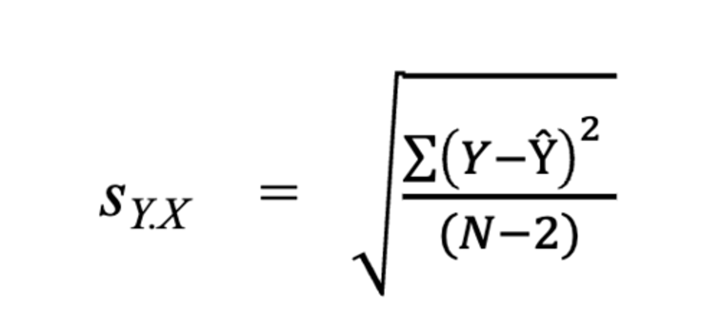
***what does the formula for linear regression represent:

based on a dataset of (X, Y) pairs, (Y – Ŷ ) is an estimation error/residual, where Y is an observed value for some X, and Ŷ is the estimated value given by the regression line for that X The SD of the residuals is written as sY.X ,and the summation is over all N data points

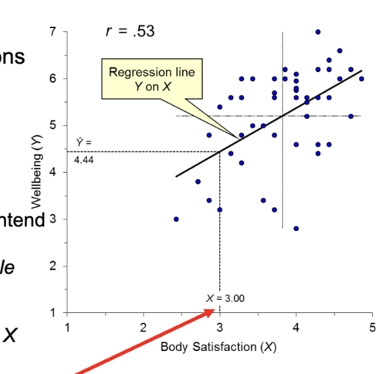
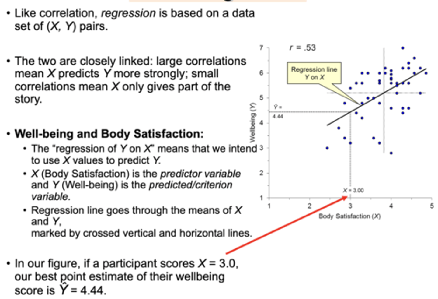
Well-being and Body Satisfaction linear regression example:

The “regression of Y on X” means that we intend to use X values to predict Y.• X (Body Satisfaction) is the predictor variable and Y (Well-being) is the predicted/criterion variable.

Regression line goes through the means of X and Y, marked by crossed vertical and horizontal lines. In our figure, if a participant scores X = 3.0, what is our best point estimate of their wellbeing score?

our best point estimate of their wellbeing score is Ŷ = 4.44

**Calculation for multiple regression:

is through partial R2

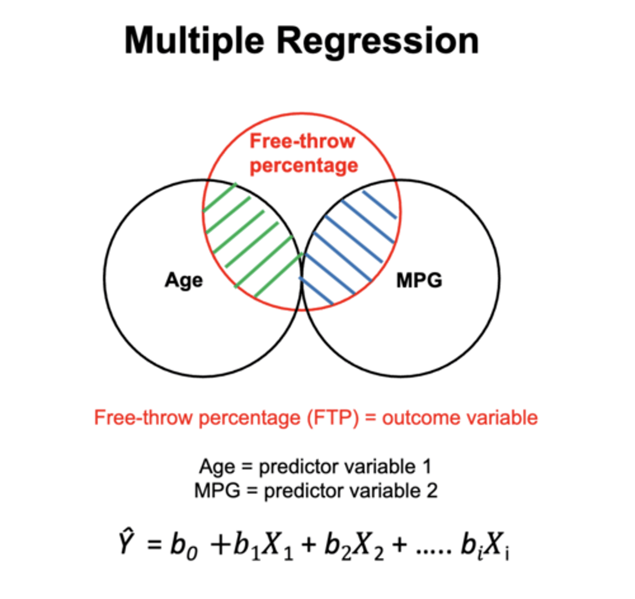
**Complications with multiple regression:

It can be confusing as there are 2 predictor variables being assessed for effects on the main outcome variable, they are both correlated but independent

***What does the formula for multiple regression represent:

using partial r2: the b's in the formula represent each predictor variable and how they are added to get overall outcome variable in percentage (how much change in the outcome variable results form one-unit of change in the predictor variable adter controlling for the other predictor variable)

FREE THROW EX: after accounting for Age, bMPG = 0.33, which means that FTP increases by 0.33% for every extra minute of game time, regardless of Age. (In other words, bmpg tells us how much FTP increases with each minute of game actionwhen we hold the age of the player constant (i.e., considering only 28-year olds)

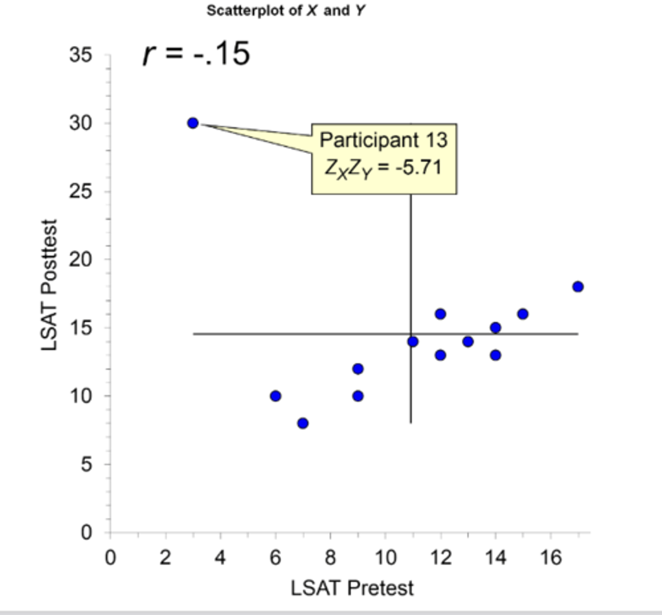
what influence does an outlier have on r?

The distance of a point from the means of X and Y tells the tale of itsinfluence on r:
• it has a much stronger contribution to r ( in fact, this single data point turned our correlation from .89 to -.15!)

what is a regression based on:

a dataset of (X, Y) pairs.• The two are closely linked: large correlations mean X predicts Y more strongly; small correlations mean X only gives part of the story.

what is an estimation error/residual

is (Y – Ŷ ) where Y is anobserved value for some X, and Ŷ is the estimated value givenby the regression line for that X (regression line minimizes this error!!)

how to find the slope of regression line:

b = r X (Sy/Sx) indicates how strongly the x and y variables are related

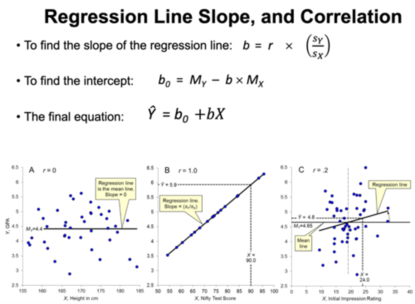
How to find the intercept of regression line:

b0 = My - b X Mx

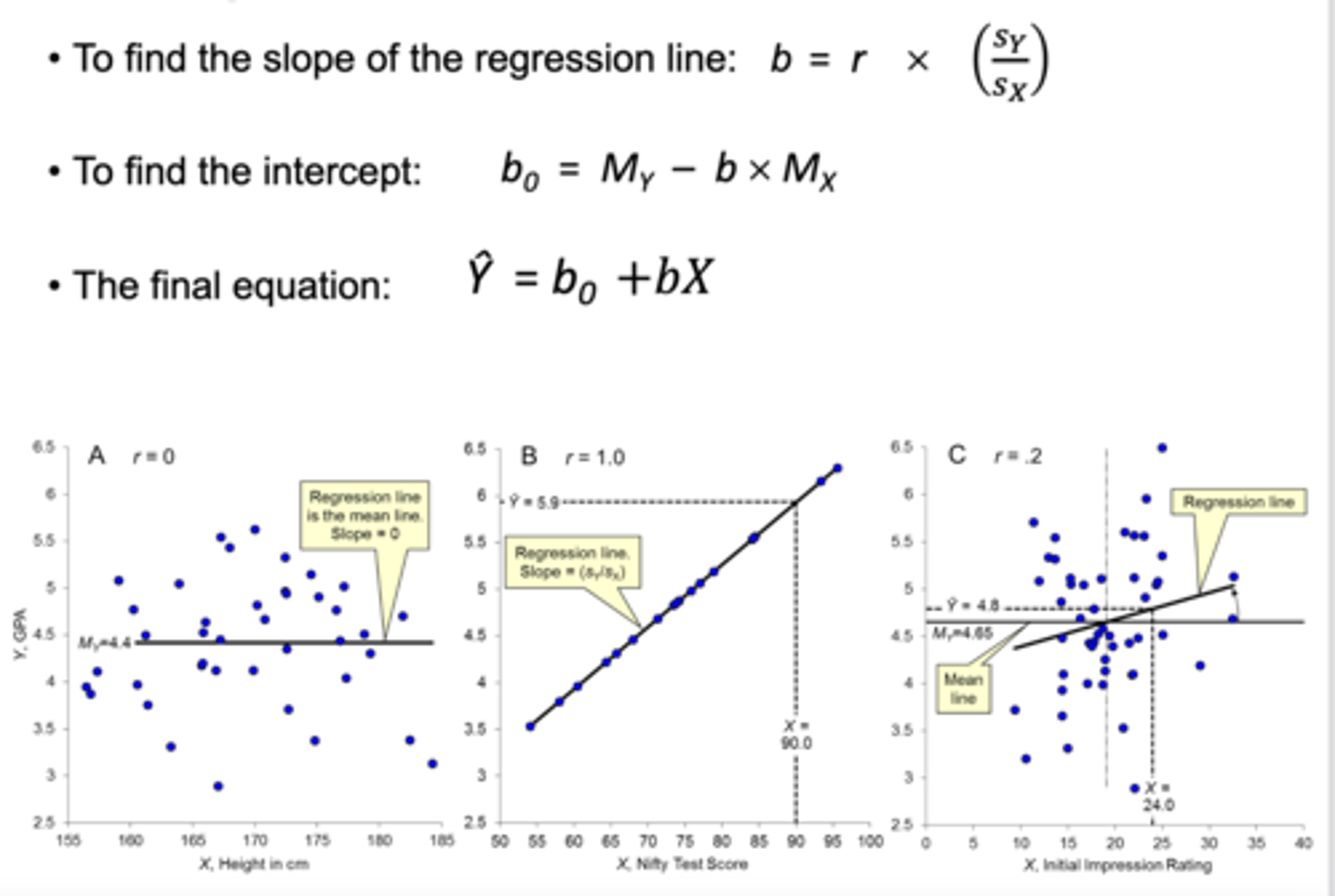
final equation of r correlation:

Ŷ = b0 +𝑏𝑋

what is the Nifty test?

a good predictor test demonstrating the relationship between 2 variables EX:The correlation coefficient (r) between predictor X ("Nifty test score") and outcome Y (GPA)

Two extreme cases of correlation:

r=0: No correlation; the regression line is flat (mean line), and knowing X provides no information about Y.

r=1: Perfect positive correlation; all data points lie on the regression line, and knowing X gives exact knowledge of Y