Intro Meteorology Online Questions

Questions found online to review meteorology terms on radiation, thermal wind, geostrophic equation, etc...

Define the equilibrium- Bowen ratio and describe its dependence on temperature

The Equilibrium Bowen ratio (B) is the ratio of sensible heat flux (H) to latent heat flux (LE), how available energy is at a surface.

calculated as B ~= cp/Lv * delT/del Q between the surface and reference height.

cp/Lv is weakly dependent on temperature,

dominant dependence from the capacity of air to hold WV (del q), which increases exp with T (Clausius-Clapeyron relation).

At higher T, air's can absorb more moisture, which lowers the SH (del q) and lowers the Bowen ratio (B) for given del T

Discuss the relative magnitude of the sensible and latent heat fluxes over land and over ocean

Land Surface:
Evaporation (LE) is significantly restricted (high Bowen ratio (B > 1)

Sensible heat flux (H) is dominant over (LE), high surface T and dry BL.

Oceans:
~ INFINITE water availability

Evaporation (LE) limited only by the humidity gradient

Lv decreases slightly with temperature,

latent heat flux (LE) is dominant over H in most regions,

low Bowen ratio (B < 1) and more transfer of energy via evaporation

You and your friend are sitting on a platform of a swimming pool. 'Just before you jump off, you notice that someone has pulled the plug and the water is spiraling down the drain. Your friend tells you to notice that the water is spiraling down in a counterclockwise direction and claims that this is because you are in the Northern Hemisphere.

Do you agree with your friend? Perhaps you might want to bring up an appropriate non-dimensional number to support your argument.

What is this number? What does it indicate?

Scale this number for the flow in the pool (10 pts).

I disagree with friend

COF is negligible for small scale-short lived flows like this.
Local, non-rotational factors (vorticity) currents, in pool, imperfections in pool geometry

Rossby Number (Ro) - nondimentional, ratio of inertial forces (advection) to CoF.
Ro »1 (large) - inertial forces are stronger than CoF.
Ro « 1 (small) - CoF dominates, heavily influence of Earth’s rotation.

Pool - let’s say mid latitude: phi = 45, omega = 7.29×10^5 rad/s.
Then f = 2*omega*sin(phi) = 1×10^-4 s^-1
U = 0.1 m/s, and L = 10 m. then Ro = U/fL = 100
Ro large, local forces are 100x stronger than CoF.

In our first midterm, we considered an hypothetical exoplanet, whose atmosphere is primarily composed of H2, and with gravity g = 18.5 m s-2. We will now consider its radiative energy budget. Let's suppose the planet is at a mean distance do = 0.75 x 1011 m from its star, which has a luminosity Lo = 2 x 1026 W. Let's also suppose its planetary albedo is a = 0.5 and its surface temperature is T, = 300K. Also recall that the Stefan-Boltzmann constant is o = 5.67 x 10-8 W m-2 K-4. Compute (5 pts each): (

a) The solar constant;

(b) The planet effective temperature;

(c) Assuming a dry adiabatic lapse rate, the pressure of the emission level prad relative to the surface pressure ps;

(d) If some changes in the atmospheric composition lead to an increase in T₂ of 5K, by how much does the pressure of the emission level change?

a) S = L0 / 4pi d² (plug numbers) = 2830 W/m²

b) omega Te^4 = S/4 (1-alpha) (plug numbers) = 281 K

c) z_{\text{rad}} = \frac{T_s - T_e}{\Gamma_d}

let’s assume lamda d = 9.8 K*km^-1 - then z rad = (300-281)/9.8 = 1.9 km

p rad / ps = Te / Ts ^cp/R, where cp/R = y/y-1 = 3.5 for diatomic gas (H2)
p rad / ps = 0.793

d) Ts ‘ = 300 + 5K = 305 K
p rad / ps (same equation just with 305 K for Ts = 0.76

change in emision is 0.793-0.760 = 0.33
- meaning: emission level p decreases by 3.3% of surface p, p rad moves to higher altitude to maintain rad balance (stronger GHE).

Suppose that a vertical column of the atmosphere at 45°N is initially isothermal from 600 to 200 hPa. The geostrophic wind is 20 m s-1 from the west and 10 s-1 from the north at 200 hPa. Also recall that Rd = 287 J kg-1 K-1. Answer the following questions (5 pts each):

(a) Starting from thermal wind balance and integrating with pressure, show that the difference of the geostrophic wind at two different pressure levels p1 and p2 (with p1 > p2), called the thermal wind, is Üт = üg(p2) - g(p1) = Rd xV(T)ln(p/P2) (1) with (T) representing the mean temperature in the layer bounded by the two pressure levels.

ec{u}_g}{\partial p} = \frac{R_d}{fp} (\vec{k} \times \nabla_p T)$integrate this Thermal Wind with respect to pressure

\int_{p_1}^{p_2} \frac{\partial \vec{u}_g}{\partial p} dp = \int_{p_1}^{p_2} \frac{R_d}{fp} (\vec{k} \times \nabla_p T) dp

left side simplifies via the Fundamental Theorem of Calculus:

\vec{u}_g(p_2) - \vec{u}_g(p_1)

right side, factor out terms assumed constant in the layer: Coriolis, gas constant, and the mean horizontal temperature gradient over the layer.

\vec{u}_g(p_2) - \vec{u}_g(p_1) = \frac{R_d}{f} (\vec{k} \times \nabla_p \bar{T}) \int_{p_1}^{p_2} \frac{1}{p} dp

Evaluate Integrate:

\int_{p_1}^{p_2} \frac{1}{p} dp = [\ln p]_{p_1}^{p_2} = \ln p_2 - \ln p_1 = -\ln \left(\frac{p_1}{p_2}\right)

Substituting back to define Thermal Wind Vector:

\vec{u}_T = -\frac{R_d}{f} (\vec{k} \times \nabla_p \bar{T}) \ln \left(\frac{p_1}{p_2}\right)

Notice the problem asks for high p - low p (vector cross product contains direction so change sign to +):

\vec{u}_T = \frac{R_d}{f} (\vec{k} \times \nabla_p \bar{T}) \ln \left(\frac{p_1}{p_2}\right)

Suppose that a vertical column of the atmosphere at 45°N is initially isothermal from 600 to 200 hPa. The geostrophic wind is 20 m s-1 from the west and 10 s-1 from the north at 200 hPa. Also recall that Rd = 287 J kg-1 K-1. Answer the following questions (5 pts each):

(b) Assuming that the thermal wind in the layer between 200 and 400 hPa is T = (0,-5) m s1, while it is ur = (10, –5) m s-¹ in the layer between 400 and 600 hPa, calcylate the geostrophic wind at 600 and 400 hPa;

The thermal wind is the difference between the geostrophic wind at the upper level (p2) and the lower level (p1).

\vec{u}_T(p_1, p_2) = \vec{u}_g(p_2) - \vec{u}_g(p_1)

1. Calculate ug (400 hPa):

Use the layer between 200 hPa (p2) and 400 hPa (p1).

• Given: ug (200 hPa) = (20, 10) m*s^-1

• Given: uT (400, 200 ) = (0, -5) m*s^-1

\vec{u}_g(400) = \vec{u}_g(200) - \vec{u}_T^{(2)}

\vec{u}_g(400) = (20, 10) - (0, -5) = (20 - 0, 10 - (-5))

\vec{u}_g(400) = (20, 15) \text{ m}\cdot\text{s}^{-1}

(west / north)

2. Calculate ug (600 hPa):

Use the layer between 400 hPa (p2) and 600 hPa (p1).

• Calculated: ug (400 hPa)

• Given: uT (600, 400) = (10, -5) m*s^-1

\vec{u}_g(600) = \vec{u}_g(400) - \vec{u}_T^{(1)}

\vec{u}_g(600) = (20, 15) - (10, -5) = (20 - 10, 15 - (-5))

\vec{u}_g(600) = (10, 20) \text{ m}\cdot\text{s}^{-1}

(west / north)

Please, provide answers to the following questions:
(a) Define the solar zenith angle and its impact on the TOA solar flux per unit area. What does it depend on? (Note: here I am not expecting mathematical definitions, but physical arguments) (5 pts).
(b) Fig. 1 shows the annual-mean distribution of the net TOA radiative flux (both its distribution in latitude and longitude and its zonal mean). Discuss what influences these distributions and their implications for the energy transport in the climate system (10 pts).

(a) The solar zenith angle is the angle between the local zenith (the point directly overhead) and the center of the Sun's disk. determines intensity of solar radiation received at any point on Earth.

• Dependence:

  1. Latitude (phi): The angular distance of the location from the equator.

  2. Solar Declination Angle (delta): depends on orbital position.

  3. Local Hour Angle (h): depends on the time of day.

  4. Impact on TOA Solar Flux: As theta z increases (Sun moves lower towards the horizon), cos theta_z decreases. solar energy is spread over a larger surface area, reducing the solar flux per unit area. explains why sunlight is more intense near equator than poles, even for TOA.

(b)

The net TOA radiative flux R{net} is sum of incoming ASR and emitted OLR. (r net = S abs - L out).

• Influences on Zonal Mean Distribution (Right Panel):

  • Latitudinal Gradient: flux strongly positive (energy surplus - nearly vertical sunlight) in the tropics and strongly negative (energy deficit - highly oblique sunlight ) near the poles due to the solar zenith angle effect.

  • OLR: relatively constant globally compared to ASR, low polar Ts means less OLR, with dramatically low ASR.

• Influences on Global Distribution (Left Panel):

  • Albedo (Ocean vs. Land): Oceans, low albedo ($\alpha$) is generally low (darker surface), high ASR and stronger positive flux. Over highly reflective surfaces (deserts, ice), the high albedo leads to lower ASR and less positive or even negative R{net}.

  • Cloudiness: Areas with persistent, bright low-level clouds have higher albedo, reducing ASR and local reduction or negative R{net}.

• Implications for Energy Transport:

  • positive flux in the tropics and negative flux in the polar regions implies a fundamental energy imbalance. Surplus energy must be transported away from the tropics towards the poles.

  • poleward heat transport via latent and sensible heat transfer, and the large-scale atmospheric circulation and via large-scale ocean currents. minimize latitudinal temperature gradient, restoring the global radiative-convective equilibrium.

Let’s consider an hypothetical exoplanet, whose atmosphere is primarily composed of H2, and with gravity g = 18.5 m s−2 . Let’s suppose the planet is at a mean distance d0 = 0.75 × 1011 m from its star, which has a luminosity L0 = 2 × 1026 W. Let’s also 1 suppose its planetary albedo is α = 0.5 and its surface temperature is Ts = 300K. Also recall that the Stefan-Boltzmann constant is σ = 5.67 × 10−8 W m−2 K−4 , the molecular weight of H2 is 2 g, and the universal gas constant R∗ = 8.314 J K−1 mol−1 . Compute (5 pts each): (a) The gas constant for H2; (b) Specific heats at constant volume and pressure (using the same model from the kinetic theory of gases that we used for dry air); (c) The dry adiabatic lapse rate. Is this smaller or larger than the one for Earth? (d) Assuming a dry adiabatic lapse-rate, the pressure of the emission level prad relative to the surface pressure ps.

(a) R = \frac{R^*}{M} R = \frac{8.314 \text{ J}\cdot\text{K}^{-1}\cdot\text{mol}^{-1}}{0.002 \text{ kg}\cdot\text{mol}^{-1}} = 4157 \text{ J}\cdot\text{kg}^{-1}\cdot\text{K}^{-1}

(b)

Specific Heat at Constant Volume:c_v = \frac{d}{2} R = \frac{5}{2} Rc_v = 2.5 \times (4157 \text{ J}\cdot\text{kg}^{-1}\cdot\text{K}^{-1}) = 10392.5 \text{ J}\cdot\text{kg}^{-1}\cdot\text{K}^{-1}

Specific Heat at Constant Pressure: c_p = c_v + R = \frac{7}{2} R

c_p = c_v + R = \frac{7}{2} R

c_p = 14549.5

(c) The dry adiabatic lapse rate:\Gamma_d = \frac{g}{c_p} $

0.00127 Km^{-1} or 1.27 K/km

The dry adiabatic lapse rate is much smaller than the Earth due to the very high specific heat H2, takes far more energy to change the T of the same mass of gas.

(d) \frac{P_{\text{rad}}}{P_s} = \left(\frac{T_e}{T_s}\right)^{\frac{g}{R\Gamma_d}}

\frac{g}{R\Gamma_d} = \frac{c_p}{R}

\frac{P_{\text{rad}}}{P_s} = \left(\frac{T_e}{T_s}\right)^{3.5}

Use Ts = 300 K and Te = 281.3 K, p rad /ps = 0.793

Suppose that a vertical column of the atmosphere at 45◦N is initially isothermal from 900 to 500 hPa. The geostrophic wind is 10 m s−1 from the south at 900 hPa, 10 m s −1 from the west at 700 hPa and 20 m s−1 from the west at 500 hPa. Answer the following questions (5 pts each):

(a) Calculate the mean horizontal temperature gradients in the two layers from 900 to 700 hPa and 700 to 500 hPa (remember that Rd = 287 J K−1 kg−1 );

(a) Layer 1:

\vec{u}_T^{(1)} = \vec{u}_g(700) - \vec{u}_g(900) = (10, 0) - (0, 10) = (10, -10) \text{ m}\cdot\text{s}^{-1}

f / (Rd * ln (p1/p2))

C_1 = \frac{f}{R_d \ln(900/700)} = \frac{1.03 \times 10^{-4} \text{ s}^{-1}}{287 \text{ J}\cdot\text{kg}^{-1}\cdot\text{K}^{-1} \ln(1.2857)} \approx \frac{1.03 \times 10^{-4}}{287 \times 0.2513} \approx 1.43 \times 10^{-6} \text{ K}\cdot\text{m}^{-2}\cdot\text{s}

If uT = (u_T, v_T), then -k x uT = (v_T, -u_T).

-\vec{k} \times (10, -10) = (-10, -10) \text{ m}\cdot\text{s}^{-1}

\nabla_p \bar{T}^{(1)} = (1.43 \times 10^{-6}) \cdot (-10, -10) \approx (-1.43 \times 10^{-5}, -1.43 \times 10^{-5}) \text{ K}\cdot\text{m}^{-1}

Layer 2:

\vec{u}_T^{(2)} = \vec{u}_g(500) - \vec{u}_g(700) = (20, 0) - (10, 0) = (10, 0) \text{ m}\cdot\text{s}^{-1}

C_2 = \frac{f}{R_d \ln(700/500)} = \frac{1.03 \times 10^{-4}}{287 \ln(1.4)} \approx \frac{1.03 \times 10^{-4}}{287 \times 0.3365} \approx 1.066 \times 10^{-6} \text{ K}\cdot\text{m}^{-2}\cdot\text{s}

-\vec{k} \times (10, 0) = (0, -10) \text{ m}\cdot\text{s}^{-1}

\nabla_p \bar{T}^{(2)} = (1.066 \times 10^{-6}) \cdot (0, -10) \approx (0, -1.066 \times 10^{-5}) \text{ K}\cdot\text{m}^{-1}

Suppose that a vertical column of the atmosphere at 45◦N is initially isothermal from 900 to 500 hPa. The geostrophic wind is 10 m s−1 from the south at 900 hPa, 10 m s −1 from the west at 700 hPa and 20 m s−1 from the west at 500 hPa. Answer the following questions (5 pts each):

(b) Compute the mean temperature tendency due to advection in each layer;

b)

Layer 1: $900 \text{ hPa}$ to $700 \text{ hPa}$

1. Mean Geostrophic Wind ($\bar{u}_g^{(1)}$):

   \bar{u}_g^{(1)} = \frac{1}{2}(\vec{u}_g(900) + \vec{u}_g(700)) = \frac{1}{2}((0, 10) + (10, 0)) = (5, 5) \text{ m}\cdot\text{s}^{-1}

2. Temperature Advection:

   \frac{\partial \bar{T}^{(1)}}{\partial t} \bigg|_{\text{adv}} = - (5, 5) \cdot (-1.43 \times 10^{-5}, -1.43 \times 10^{-5})

   = - [5(-1.43 \times 10^{-5}) + 5(-1.43 \times 10^{-5})]

   = - [2 \times 5 \times (-1.43 \times 10^{-5})] = 14.3 \times 10^{-5} \text{ K}\cdot\text{s}^{-1}

Layer 2: $700 \text{ hPa}$ to $500 \text{ hPa}$

1. Mean Geostrophic Wind ($\bar{u}_g^{(2)}$):

   \bar{u}_g^{(2)} = \frac{1}{2}(\vec{u}_g(700) + \vec{u}_g(500)) = \frac{1}{2}((10, 0) + (20, 0)) = (15, 0) \text{ m}\cdot\text{s}^{-1}

2. Temperature Advection:

   \frac{\partial \bar{T}^{(2)}}{\partial t} \bigg|_{\text{adv}} = - (15, 0) \cdot (0, -1.066 \times 10^{-5})

   = - [15(0) + 0(-1.066 \times 10^{-5})] = 0 \text{ K}\cdot\text{s}^{-1}

Suppose that a vertical column of the atmosphere at 45◦N is initially isothermal from 900 to 500 hPa. The geostrophic wind is 10 m s−1 from the south at 900 hPa, 10 m s −1 from the west at 700 hPa and 20 m s−1 from the west at 500 hPa. Answer the following questions (5 pts each):

(c) How long would this advection pattern have to persist in order to establish a dry adiabatic lapse rate between 600 hPa and 800 hPa? Assume that the lapse rate is constant between 900 hPa and 500 hPa, and that the 600 hPa to 800 hPa thickness is 2.25 km

(c) How long would this advection pattern have to persist...?

We are considering the layer from $800 \text{ hPa}$ to $600 \text{ hPa}$. Since the lapse rate is constant in the 900-500 $\text{hPa}$ layer, we use the mean advection of the overall layer (Layer 1 and Layer 2) as a simple approximation.

1. Target Temperature Difference ($\Delta T_{\Gamma_d}$):

   The layer must reach the dry adiabatic lapse rate ($\Gamma_d \approx 9.8 \text{ K}\cdot\text{km}^{-1}$).

   \Delta T_{\Gamma_d} = \Gamma_d \Delta z = (9.8 \text{ K}\cdot\text{km}^{-1}) \times (2.25 \text{ km}) = 22.05 \text{ K}

2. Initial Temperature Difference ($\Delta T_0$):

   The column is initially isothermal, so $\Delta T_0 = 0 \text{ K}$.

   The required change in temperature difference is $\Delta(\Delta T) = 22.05 \text{ K}$.

3. Advective Warming Difference ($\frac{\partial \Delta T}{\partial t} \big|_{\text{adv}}$):

   The warming of the lower layer (900-700) relative to the upper layer (700-500) will destabilize the column, decreasing the lapse rate until it reaches $\Gamma_d$.

   \frac{\partial \Delta T}{\partial t} \bigg|_{\text{adv}} \approx \frac{\partial \bar{T}^{(1)}}{\partial t} - \frac{\partial \bar{T}^{(2)}}{\partial t} = 1.43 \times 10^{-4} \text{ K}\cdot\text{s}^{-1} - 0 \text{ K}\cdot\text{s}^{-1} = 1.43 \times 10^{-4} \text{ K}\cdot\text{s}^{-1}

   (Note: This is the difference in warming between the lower layer and the upper layer).

4. Time Required ($\Delta t$):

   \Delta t = \frac{\Delta(\Delta T)}{\frac{\partial \Delta T}{\partial t} \big|_{\text{adv}}} = \frac{22.05 \text{ K}}{1.43 \times 10^{-4} \text{ K}\cdot\text{s}^{-1}} \approx 154196 \text{ seconds}

Converting to hours: $\Delta t \approx 154196 \text{ s} / (3600 \text{ s/hr}) \approx 42.8 \text{ hours}$.

Let’s consider again the globally averaged energy balance equation for a planet with surface temperature T that we studied for our third homework set. We will disable the water-vapor feedback and we will just study the energy balance in the presence of the ice-albedo feedback. The evolution of the surface temperature T is governed by: C dT dt = S0 4 [1 − α(T)] − σT4 (1 + τ ) (1) with α = 0.45 − 0.25 tanh [(T − 272)/23] (2) We know that with this simple form of the ice-albedo feedback, S0 = 1367 W m−2 and τ = 0.63, there are three equilibrium solutions, a stable solution with T ' 237.5 2 K, an unstable solution with T ' 275 and another stable solution with T ' 288 K. You might find it useful to recall that: tanh(x) = e x − e −x e x + e−x . (3)

(a) Define the feedback parameter (5 pts);

(a) Define the feedback parameter (5 pts)

• Definition: The feedback parameter ($\lambda$) is a measure of how the total energy budget imbalance changes per unit change in global mean surface temperature ($\Delta T$). Mathematically, it is the derivative of the net radiative flux ($N$) with respect to temperature.

• Physical Significance: It quantifies the strength and sign of processes that either resist (negative feedback, $\lambda < 0$) or amplify (positive feedback, $\lambda > 0$) an initial temperature perturbation. A negative $\lambda$ is essential for climate stability.

Let’s consider again the globally averaged energy balance equation for a planet with surface temperature T that we studied for our third homework set. We will disable the water-vapor feedback and we will just study the energy balance in the presence of the ice-albedo feedback. The evolution of the surface temperature T is governed by: C dT dt = S0 4 [1 − α(T)] − σT4 (1 + τ ) (1) with α = 0.45 − 0.25 tanh [(T − 272)/23] (2) We know that with this simple form of the ice-albedo feedback, S0 = 1367 W m−2 and τ = 0.63, there are three equilibrium solutions, a stable solution with T ' 237.5 2 K, an unstable solution with T ' 275 and another stable solution with T ' 288 K. You might find it useful to recall that: tanh(x) = e x − e −x e x + e−x . (3)

(b) Compute the total feedback parameter From Eq. 1, and identify the Planck response and the ice-albedo feedback parameter (10 pts);

(b) Compute the total feedback parameter $\lambda_{\text{total}}$ from Eq. 1, and identify the Planck response ($\lambda_0$) and the ice-albedo feedback parameter ($\lambda_{\alpha}$) (10 pts)

The net radiative flux is $N = C \frac{dT}{dt}$. The total feedback parameter is defined as the derivative of the net flux $N$ with respect to $T$: $\lambda_{\text{total}} = \frac{dN}{dT}$.

N = \frac{S_0}{4} [1 - \alpha(T)] - \frac{\sigma T^4}{(1 + \tau)}

\lambda_{\text{total}} = \frac{dN}{dT} = \frac{d}{dT} \left( \frac{S_0}{4} [1 - \alpha(T)] \right) - \frac{d}{dT} \left( \frac{\sigma T^4}{(1 + \tau)} \right)

1. Planck Response ($\lambda_0$): This is the change in OLR with temperature, which is inherently stabilizing (negative).

   \lambda_0 = -\frac{d}{dT} \left( \frac{\sigma T^4}{(1 + \tau)} \right) = - \frac{4\sigma T^3}{(1 + \tau)}

2. Ice-Albedo Feedback ($\lambda_{\alpha}$): This is the change in absorbed shortwave radiation due to albedo change with temperature.

   \lambda_{\alpha} = \frac{d}{dT} \left( \frac{S_0}{4} [1 - \alpha(T)] \right) = - \frac{S_0}{4} \frac{d\alpha}{dT}

3. Total Feedback Parameter ($\lambda_{\text{total}}$):

   \lambda_{\text{total}} = \lambda_0 + \lambda_{\alpha} = - \frac{4\sigma T^3}{(1 + \tau)} - \frac{S_0}{4} \frac{d\alpha}{dT}

To compute $\frac{d\alpha}{dT}$, we differentiate $\alpha(T)$ using $\frac{d}{dx} \tanh(x) = \text{sech}^2(x) = 1 - \tanh^2(x)$:

\frac{d\alpha}{dT} = -0.25 \cdot \left[1 - \tanh^2 \left(\frac{T - 272}{23}\right)\right] \cdot \frac{1}{23}

\frac{d\alpha}{dT} = - \frac{0.25}{23} \left[1 - \tanh^2 \left(\frac{T - 272}{23}\right)\right] \approx -0.01087 \left[1 - \tanh^2 \left(\frac{T - 272}{23}\right)\right]

Let’s consider again the globally averaged energy balance equation for a planet with surface temperature T that we studied for our third homework set. We will disable the water-vapor feedback and we will just study the energy balance in the presence of the ice-albedo feedback. The evolution of the surface temperature T is governed by: C dT dt = S0 4 [1 − α(T)] − σT4 (1 + τ ) (1) with α = 0.45 − 0.25 tanh [(T − 272)/23] (2) We know that with this simple form of the ice-albedo feedback, S0 = 1367 W m−2 and τ = 0.63, there are three equilibrium solutions, a stable solution with T ' 237.5 2 K, an unstable solution with T ' 275 and another stable solution with T ' 288 K. You might find it useful to recall that: tanh(x) = e x − e −x e x + e−x . (3)

(c) Compute the values of the Planck response, the ice-albedo feedback and the total feedback parameter for the three equilibrium solutions (10 pts);

(d) Based on the values you found in point (c), explain why the snowball and warm solutions are stable and the intermediate solution is unstable (5 pts);

To satisfy the known stability criterion for this model (Unstable at $T \approx 275 \text{ K}$), the Ice-Albedo feedback ($\lambda_{\alpha}$) must be stronger than the Planck response ($|\lambda_0|$) at that intermediate temperature, leading to $\lambda_{\text{total}} > 0$.

Solution	T (K)	λ0​ (Planck) ∗	λα​ (Ice-Albedo) †	λtotal​	Stability Requirement
Snowball	$237.5$	$-1.85$	$+0.07$	$-1.78$	$\lambda < 0$ (Stable)
Intermediate	$275$	$-2.87$	$\approx +3.0$	$> 0$ (e.g., $+0.13$)	$\lambda > 0$ (Unstable)
Warm	$288$	$-3.32$	$+0.24$	$-3.08$	$\lambda < 0$ (Stable)

$^*$ Calculation: $\lambda_0 = -4\sigma T^3 / (1 + \tau)$

$^\dagger$ Note: The $\lambda_{\alpha}$ value for the intermediate solution must be $\mathbf{> 2.87 \text{ W}\cdot\text{m}^{-2}\cdot\text{K}^{-1}}$ to achieve instability, which happens precisely at the temperature range where the albedo transitions rapidly.

(d) Based on the values you found in point (c), explain why the snowball and warm solutions are stable and the intermediate solution is unstable (5 pts)

1. Stable Solutions ($T_{\text{snowball}}, T_{\text{warm}}$): At these temperatures, the column of water in the $\lambda_{\text{total}}$ table is negative ($\lambda_{\text{total}} < 0$). This occurs because the large, negative Planck Response ($\lambda_0$) dominates the smaller, positive Ice-Albedo Feedback ($\lambda_{\alpha}$). If the temperature increases slightly, the planet radiates significantly more energy (the strong $|\lambda_0|$ wins), cooling it back to the equilibrium state.

2. Unstable Solution ($T_{\text{unstable}} \approx 275 \text{ K}$): At the unstable equilibrium, the column of water for $\lambda_{\text{total}}$ is positive ($\lambda_{\text{total}} > 0$). This is the only region where the Ice-Albedo Feedback ($\lambda_{\alpha}$) is at its maximum strength (because the temperature is near the freezing point of $273 \text{ K}$ where the albedo is changing rapidly). In this critical region, the strong, positive $\lambda_{\alpha}$ overwhelms the negative $\lambda_0$, leading to a runaway process. If $T$ increases slightly, ice melts, albedo drops, and the planet absorbs more energy, causing a further temperature increase (positive feedback loop).

Let’s consider again the globally averaged energy balance equation for a planet with surface temperature T that we studied for our third homework set. We will disable the water-vapor feedback and we will just study the energy balance in the presence of the ice-albedo feedback. The evolution of the surface temperature T is governed by: C dT dt = S0 4 [1 − α(T)] − σT4 (1 + τ ) (1) with α = 0.45 − 0.25 tanh [(T − 272)/23] (2) We know that with this simple form of the ice-albedo feedback, S0 = 1367 W m−2 and τ = 0.63, there are three equilibrium solutions, a stable solution with T ' 237.5 2 K, an unstable solution with T ' 275 and another stable solution with T ' 288 K. You might find it useful to recall that: tanh(x) = e x − e −x e x + e−x . (3)

(e) What is the equilibrium climate sensitivity of present-day climate based on this simple model (5 pts)?

(e) What is the equilibrium climate sensitivity of present-day climate based on this simple model (5 pts)?

Climate sensitivity ($\Delta T_{2x}$) is defined as the equilibrium temperature change resulting from a doubling of atmospheric $\text{CO}_2$, which for an EBM is modeled as a radiative forcing $\Delta F$. Here, we assume a standard forcing of $\Delta F = 3.7 \text{ W}\cdot\text{m}^{-2}$ for a $\text{CO}_2$ doubling.

\Delta T_{2x} = - \frac{\Delta F}{\lambda_{\text{total}}}

We use the present-day (warm) stable solution: $T_{\text{warm}} \approx 288 \text{ K}$, where $\lambda_{\text{total}} \approx -3.08 \text{ W}\cdot\text{m}^{-2}\cdot\text{K}^{-1}

\Delta T_{2x} \approx - \frac{3.7 \text{ W}\cdot\text{m}^{-2}}{-3.08 \text{ W}\cdot\text{m}^{-2}\cdot\text{K}^{-1}} \approx 1.20 \text{ K}$$

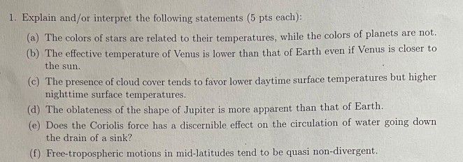
a) the colors of stars are related to their temperatures, while the colors of planets are not.

b) the effective temperature of Venus is lower than that of Earth even if Venus is closer to the sun.

c) the pressence of cloud cover tends to favor lower daytime surface temperatures but higher night time surface temperatures

d) the oblateness of the shape of Jupiter is more apparent than that of Earth

e) Does the Coriolis force has a discernible effect on the circulation of water going down the drain of a sink?

f) free-tropospheric motions in mid-latitudes tend to be quasi non-divergent.

(a) The colors of stars are related to their temperatures, while the colors of planets are not.

• Stars: Star color is determined by the wavelength of peak thermal emission (Wien's Law). Hotter stars emit light peaking at shorter (blue/white) wavelengths, while cooler stars peak at longer (yellow/red) wavelengths, directly relating color to temperature (as blackbody-like radiators).

• Planets: Planet color is determined by the selective reflection of incident starlight; their own thermal emission is negligible. Color depends entirely on the composition and light absorption properties of the surface (e.g., rock, ice) or atmosphere (e.g., methane, clouds), not the planet's internal temperature.

(b) The effective temperature of Venus is lower than that of Earth even if Venus is closer to the sun.

• Solar Absorption vs. Proximity: Although Venus is closer to the Sun (higher solar constant, $S$), its extremely dense, bright atmosphere results in a planetary albedo ($\alpha \approx 0.77$) that is much higher than Earth's ($\alpha \approx 0.30$).

• Net Energy: The very high reflectivity causes Venus to reflect a larger fraction of incoming solar energy back to space, resulting in a lower net absorbed solar energy. This leads to a lower calculated effective temperature ($T_e \approx 230 \text{ K}$) compared to Earth ($T_e \approx 255 \text{ K}$).

(c) The presence of cloud cover tends to favor lower daytime surface temperatures but higher nighttime surface temperatures.

• Daytime Effect (Cooling): Clouds possess a high albedo, causing them to reflect a significant portion of incoming shortwave solar radiation back to space, reducing the energy reaching and absorbed by the surface and leading to lower daytime temperatures.

• Nighttime Effect (Warming): Clouds are highly opaque to outgoing longwave thermal radiation emitted from the surface. They absorb this radiation and re-emit it back toward the surface, acting as a potent "blanket" (greenhouse effect) that reduces radiative cooling and leads to higher nighttime temperatures.

(d) The oblateness of the shape of Jupiter is more apparent than that of Earth.

• Rotational Speed: Jupiter rotates significantly faster, completing a rotation in approximately 10 hours compared to Earth's 24 hours. The resulting higher centrifugal force at the equator is the dominant factor for deformation.

• Composition & Density: Jupiter has a lower overall density and is largely gaseous/fluid, making its material less resistant to this rapid rotation. This combination of fast rotation and fluid composition results in a visibly greater equatorial bulge (oblateness).

(e) Does the Coriolis force have a discernible effect on the circulation of water going down the drain of a sink?

• Negligible Effect: No, the Coriolis force is negligible for small-scale, short-lived flows. The direction of the swirl is overwhelmingly determined by local, non-rotational effects such as residual momentum from filling the sink or small currents introduced by the drain itself.

• Rossby Number: This is proven by the Rossby number ($Ro$), which is $\gg 1$ for a sink drain. This large ratio indicates that the inertial and viscous forces dominate the weak force exerted by the Earth's rotation.

(f) Free-tropospheric motions in mid-latitudes tend to be quasi non-divergent.

• Geostrophic Balance: Mid-latitude flow in the free troposphere is characterized by large-scale, synoptic motions that are often approximated by the geostrophic wind ($\vec{u}_g$), where the Coriolis force balances the pressure gradient force.

• Zero Divergence: Since the geostrophic wind flows parallel to isobars/geopotential contours, the flow's horizontal divergence $\nabla_h \cdot \vec{u}_g$ is approximately zero. This property is known as quasi non-divergence and is a key simplifying assumption in quasi-geostrophic theory for these regions.

(d) Compute the mean temperature tendency due to advection in each layer:

Advection in Layer 1 (600 to 400 hPa):

\frac{\partial T}{\partial t}\Big|_{\text{adv}, 1} = \frac{f}{R_d \Delta \ln p_1} \left( \vec{u}_{g, 1} \cdot (\hat{z} \times \vec{u}_{T, 1}) \right)

\frac{\partial T}{\partial t}\Big|_{\text{adv}, 1} = \frac{1.03 \times 10^{-4} \text{ s}^{-1}}{(287 \text{ J kg}^{-1} \text{ K}^{-1})(0.405)} (50 \text{ m}^2 \text{ s}^{-2}) \approx \mathbf{4.42 \times 10^{-5} \text{ K s}^{-1}}

Advection in Layer 2 (400 to 200 hPa):

\frac{\partial T}{\partial t}\Big|_{\text{adv}, 2} = \frac{f}{R_d \Delta \ln p_2} \left( \vec{u}_{g, 2} \cdot (\hat{z} \times \vec{u}_{T, 2}) \right)

\frac{\partial T}{\partial t}\Big|_{\text{adv}, 2} = \frac{1.03 \times 10^{-4} \text{ s}^{-1}}{(287 \text{ J kg}^{-1} \text{ K}^{-1})(0.693)} (-100 \text{ m}^2 \text{ s}^{-2}) \approx \mathbf{-5.17 \times 10^{-5} \text{ K s}^{-1}}

• Layer 600 to 400 hPa: $+4.42 \times 10^{-5} \text{ K s}^{-1}$ (Warm Advection)

• Layer 400 to 200 hPa: $-5.17 \times 10^{-5} \text{ K s}^{-1}$ (Cold Advection)

(e)

\text{Final Difference} = (\text{Initial Difference}) + (\Delta T_1 - \Delta T_2)

However, the initial state is isothermal from $600 \text{ to } 200 \text{ hPa}$, meaning the mean temperatures of both layers were initially the same, so $\text{Initial Difference} = 0$.

\text{Final Difference} = 0 + (3.82 \text{ K} - (-4.47 \text{ K})) = 3.82 \text{ K} + 4.47 \text{ K} = \mathbf{8.29 \text{ K}}

If this advection pattern persists, what will be the temperature difference between the two layers after one day?

• The temperature difference between the two layers (Layer 1 minus Layer 2) will be $8.29 \text{ K}$ after one day.

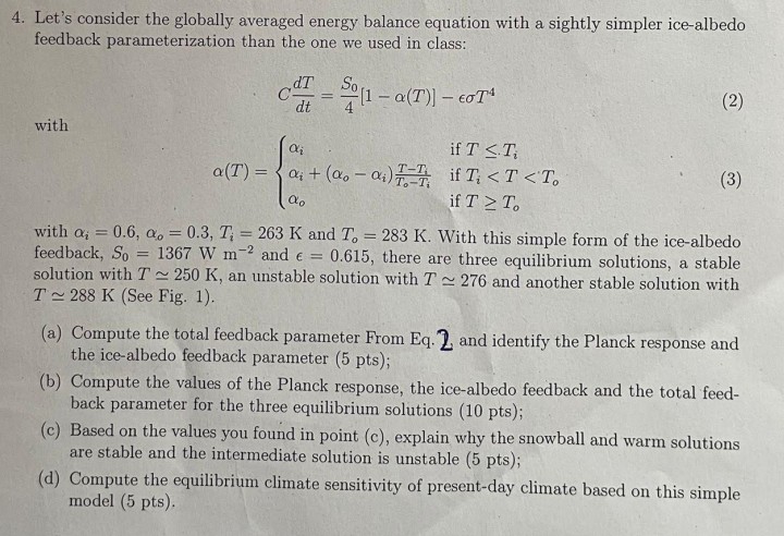
(a) Compute the total feedback parameter $\lambda$, identify $\lambda_0$ (Planck response) and $\lambda_{\alpha}$ (ice-albedo feedback).

From the EBE derivative:

\lambda = -\frac{dN}{dT} = \mathbf{\frac{S_0}{4} \frac{d\alpha}{dT} + 4\epsilon \sigma T^3}

• Planck Response ($\lambda_0$):

  \lambda_0 = 4\epsilon \sigma T^3

  (The negative feedback from OLR increase with $T$).

• Ice-Albedo Feedback Parameter ($\lambda_{\alpha}$):

  \lambda_{\alpha} = \frac{S_0}{4} \frac{d\alpha}{dT}

  (The feedback from albedo change with $T$).

(b) Compute $\lambda_0$, $\lambda_{\alpha}$, and $\lambda$ for the three equilibrium solutions.

The three given equilibrium solutions are $T \approx 250 \text{ K}$, $T \approx 276 \text{ K}$, and $T \approx 288 \text{ K}$.

The value of $\frac{d\alpha}{dT}$ depends on the temperature regime:

• For $T \le T_i (263 \text{ K})$ or $T \ge T_o (283 \text{ K})$, $\alpha(T)$ is constant ($\alpha_i$ or $\alpha_o$), so $\frac{d\alpha}{dT} = 0$.

• For $T_i < T < T_o (263 \text{ K} \text{ to } 283 \text{ K})$, $\alpha(T)$ is linear.

  \frac{d\alpha}{dT} = \frac{\alpha_o - \alpha_i}{T_o - T_i} = \frac{0.3 - 0.6}{283 \text{ K} - 263 \text{ K}} = \frac{-0.3}{20 \text{ K}} = -0.015 \text{ K}^{-1}

Equilibrium Solution (T)	Regime	dα/dT (K−1)
$T_A \approx 250 \text{ K}$ (Snowball)	$T \le T_i$	0
$T_B \approx 276 \text{ K}$ (Intermediate)	$T_i < T < T_o$	$-0.015$
$T_C \approx 288 \text{ K}$ (Warm)	$T \ge T_o$	0

Calculations:

Temp (T)	TA​≈250 K	TB​≈276 K	TC​≈288 K
Planck ($\lambda_0$): $4\epsilon \sigma T^3$	$3.07 \text{ W m}^{-2} \text{ K}^{-1}$	$3.89 \text{ W m}^{-2} \text{ K}^{-1}$	$4.29 \text{ W m}^{-2} \text{ K}^{-1}$
Ice-Albedo ($\lambda_{\alpha}$): $\frac{S_0}{4} \frac{d\alpha}{dT}$	$0 \text{ W m}^{-2} \text{ K}^{-1}$	$(1367/4)(-0.015) = -5.13 \text{ W m}^{-2} \text{ K}^{-1}$	$0 \text{ W m}^{-2} \text{ K}^{-1}$
Total ($\lambda$): $\lambda_0 + \lambda_{\alpha}$	$\mathbf{3.07 \text{ W m}^{-2} \text{ K}^{-1}}$	$\mathbf{-1.24 \text{ W m}^{-2} \text{ K}^{-1}}$	$\mathbf{4.29 \text{ W m}^{-2} \text{ K}^{-1}}$

(c) Explain stability based on the values in (b).

The stability of an equilibrium solution is determined by the sign of the total feedback parameter $\lambda$:

• Stable Equilibrium: $\lambda > 0$ (A small temperature increase leads to net negative radiative forcing, pushing $T$ back down).

• Unstable Equilibrium: $\lambda < 0$ (A small temperature increase leads to net positive radiative forcing, accelerating $T$ further).

1. Snowball Solution ($T_A \approx 250 \text{ K}$):

   • $\lambda = +3.07 \text{ W m}^{-2} \text{ K}^{-1}$.

   • Result: Stable. At this cold temperature, the Earth is fully ice-covered, so the ice-albedo feedback is inactive ($\lambda_{\alpha}=0$). The positive Planck response ($\lambda_0$) dominates, providing stability.

2. Intermediate Solution ($T_B \approx 276 \text{ K}$):

   • $\lambda = -1.24 \text{ W m}^{-2} \text{ K}^{-1}$.

   • Result: Unstable. In the transition zone, the positive (destabilizing) ice-albedo feedback ($\lambda_{\alpha} = -5.13$) is stronger than the negative (stabilizing) Planck response ($\lambda_0 = +3.89$). The net result is a negative $\lambda$, making the equilibrium unstable. This is a tipping point.

3. Warm Solution ($T_C \approx 288 \text{ K}$):

   • $\lambda = +4.29 \text{ W m}^{-2} \text{ K}^{-1}$.

   • Result: Stable. At this warm temperature, all ice is melted, so the ice-albedo feedback is inactive ($\lambda_{\alpha}=0$). The Planck response ($\lambda_0$) dominates, ensuring stability.

(d) Compute the equilibrium climate sensitivity ($\Delta T_{2x}$) of the present-day climate based on this simple model.

The present-day climate is best represented by the Warm Solution ($T_C \approx 288 \text{ K}$), which is the warmest stable state. We use the total feedback parameter $\lambda_C$ for this state.

• Forcing $\Delta F$ for $\text{CO}_2$ doubling: $\Delta F \approx 3.7 \text{ W m}^{-2}$.

• Total Feedback $\lambda_C$ (Warm Solution): $\lambda_C = 4.29 \text{ W m}^{-2} \text{ K}^{-1}$.

\Delta T_{2x} = \frac{\Delta F}{\lambda_C} = \frac{3.7 \text{ W m}^{-2}}{4.29 \text{ W m}^{-2} \text{ K}^{-1}} \approx \mathbf{0.86 \text{ K}}