Cumulative AP Exam Study Guide

Statistics

The science of collecting, analyzing, and drawing conclusions from data

Descriptive Statistics

Methods of organizing and summarizing statistics

Inferential Statistics

Making generalizations from a sample to the population

Population

An entire collection of individuals or objects

Sample

A subset of the population selected for study

Variable

Any characteristic whose value changes

Data

Observations on single or multi-variables

Categorical Variables (Qualitative)

Basic characteristics

Numerical Variables (Quantitative)

Measurements or observations of numerical data

Discrete Variables

Listable sets (counts)

Continuous Variables

Any value over an interval of values (measurements)

Univariate

One variable

Bivariate

Two variables

Multivariate

Many variables

Symmetrical Distribution

Data on which both sides are fairly the same shape and size (“Bell Curve”)

Uniform Distribution

Every class has an equal frequency (number) → “a rectangle”

Skewed Distribution

One side (tail) is longer than the other side. The skewness is in the direction that the tail points (left or right)

Bimodal Distribution

Data of two or more classes have large frequencies separated by another class between them (“double hump camel”)

How to describe numerical graphs

• Shape - overall type (symmetrical, skewed right left, uniform, or bimodal)

• Outliers - gaps, clusters, etc.

• Center - middle of the data (mean, median, and mode)

• Spread - refers to variability (range, standard deviation, and IQR)

Everything must be in context to the data and situation of the graph. When comparing two distributions – MUST use comparative language!

Parameter

Value of a population (typically unknown)

Statistic

A calculated value about a population from a sample(s)

Measures of Center

• Median - the middle point of the data (50th percentile) when the data is in numerical order. If two values are present, then average them together.

• Mean - μ is for a population (parameter) and x is for a sample (statistic).

• Mode - occurs the most in the data. There can be more then one mode, or no mode at all if all data points occur once.

Variability

Allows statisticians to distinguish between usual and unusual occurrences

Measures of Spread (variability)

• Range - a single value (Max-Min)

• IQR - interquartile range (Q3 – Q1)

• Standard deviation - σ for population (parameter) & s for sample (statistic) – measures the typical or average deviation of observations from the mean – sample standard deviation is divided by df = n-1

  *Sum of the deviations from the mean is always zero!

• Variance - standard deviation squared

Resistant

Not affected by outliers

• Median

• IQR

Non-Resistant

• Mean

• Range

• Variance

• Standard Deviation

• Correlation Coefficient (r)

• Least Squares Regression Line (LSRL)

• Coefficient of Determination (r²)

Comparison of mean & median based on graph type

The mean is always pulled in the direction of the skew away from the median

Symmetrical

Mean and the median are the same value

Skewed Right

Mean is a larger value than the median

Skewed Left

The mean is smaller than the median

Trimmed Mean

Use a % to take observations away from the top and bottom of the ordered data. This possibly eliminates outliers

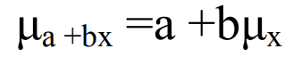
The mean is changed by both addition (subtract) & multiplication (division)

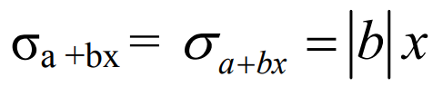
The standard deviation is changed by multiplication (division) ONLY

Just add or subtract the two (or more) means

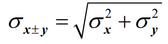
Always add the variances – X & Y MUST be independent

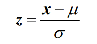
Z-Score

A standardized score. This tells you how many standard deviations from the mean an observation is. It creates a standard normal curve consisting of z-scores with a μ = 0 & σ = 1.

Normal Curve

Bell shaped and symmetrical curve.

• As σ increases the curve flattens.

• As σ decreases the curve thins.

Empirical Rule

(68-95-99.7) measures 1σ, 2σ, and 3σ on normal curves from a center of μ.

• 68% of the population is between -1σ and 1σ

• 95% of the population is between -2σ and 2σ

• 99.7% of the population is between -3σ and 3σ

Boxplots

Are for medium or large numerical data. It does not contain original observations.

• Always use modified boxplots where the fences are 1.5 IQRs from the ends of the box (Q1 & Q3). Points outside the fence are considered outliers.

• Whiskers extend to the smallest & largest observations within the fences.

5-Number Summary

1. Minimum

2. Q1 (1st Quartile – 25th Percentile)

3. Median

4. Q3 (3rd Quartile – 75th Percentile)

5. Maximum

Sample Space

Collection of all outcomes.

Event

Any sample of outcomes.

Complement

All outcomes not in the event.

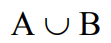
Union

A or B, all the outcomes in both circles.

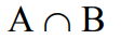
Intersection

A and B, happening in the middle of A and B.

Mutually Exclusive (Disjoint)

A and B have no intersection. They cannot happen at the same time.

Independent

If knowing one event does not change the outcome of another

Experimental Probability

The number of success from an experiment divided by the total amount from the experiment.

Law of Large Numbers

As an experiment is repeated the experimental probability gets closer and closer to the true (theoretical) probability. The difference between the two probabilities will approach “0”.

Probability Rules

• All values are 0 < P < 1.

• Probability of sample space is 1.

• P (at least 1 or more) = 1 – P (none)

Compliment of a Probability

P + (1 - P) = 1

Addition of Probabilities

P(A or B) = P(A) + P(B) – P(A & B)

Multiplication of Probabilities

P(A & B) = P(A) · P(B)

• If a & B are independent

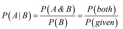
Conditional Probability

Takes into account a certain condition.

Correlation Coefficient (r)

A quantitative assessment of the strength and direction of a linear relationship. (use ρ (rho) for population parameter)

• There is a strength, direction, linear association between x & y.

• 0 → no correlation

• (0, ±0.5) → weak

• [±0.5, ±0.8) → moderate

• [±0.8, ±1] → strong

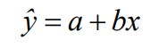
Least Squares Regression Line (LSRL)

A line of mathematical best fit. Minimizes the deviations (residuals) from the line. Used with bivariate data.

• x is independent, the explanatory variable & y is dependent, the response variable

Residuals (error)

Vertical difference of a point from the LSRL. All residuals sum up to “0”.

Residual Plot

Scatterplot of (x (or ˆy) , residual). No pattern indicates a linear relationship.

Coefficient of Determination (r²)

Gives the proportion of variation in y (response) that is explained by the relationship of (x, y). Never use the adjusted r².

• Approximately r²% of the variation in y can be explained by the LSRL of x any y.

Slope (b)

For unit increase in x, then the y variable will increase/decrease slope amount.

Extrapolation

LRSL cannot be used to find values outside of the range of the original data.

Influential Points

Points that if removed significantly change the LSRL.

Outliers

Points with large residuals.

Census

A complete count of the population.

• Why not to use a census?

  • Expensive

  • Impossible to do

  • If destructive sampling you get extinction

Sampling Frame

A list of everyone in the population.

SRS (Simple Random Sample)

One chooses so that each unit has an equal chance and every set of units has an equal chance of being selected.

• Advantages: easy and unbiased.

• Disadvantages: large σ² and must know population.

Stratified

Divide the population into homogeneous groups called strata, then SRS each strata.

• Advantages: more precise than an SRS and cost reduced if strata already available.

• Disadvantages: difficult to divide into groups, more complex formulas & must know population.

Systematic

Use a systematic approach (every 50th) after choosing randomly where to begin.

• Advantages: unbiased, the sample is evenly distributed across population & don’t need to know population.

• Disadvantages: a large σ² and can be confounded by trends.

Cluster Sample

Based on location. Select a random location and sample ALL at that location.

• Advantages: cost is reduced, is unbiased & don’t need to know population.

• Disadvantages: May not be representative of population and has complex formulas.

Random Digit Table

Each entry is equally likely and each digit is independent of the rest.

Random # Generator

Calculator or computer program

Bias

Error that favors a certain outcome, has to do with center of sampling distributions – if centered over true parameter then considered unbiased

Voluntary Response

People choose themselves to participate.

Convenience Sampling

Ask people who are easy, friendly, or comfortable asking.

Undercoverage

Some group(s) are left out of the selection process.