Empirical Research Methods

What are the four goals of empirical research?

Description, prediction, explanation, control

What are the steps of the hypothetico-deductive model?

1. Hypothesis (theory)

2. Research design (deduction)

3. Selection of possible measurements

4. Data collection (empirical)

5. Data analysis (induction)

6. Inference

7. Refine theory

What is the difference between deduction and induction?

• Deduction: take a theory, define something specific, and make it testable

• Induction: reflect on the theory based on the results of the experiment

What are the three criteria for establishing a casual relationship between two variables?

• correlation of variables

• assumed cause comes before the effect

• exclude alternative explanations

What are three methodological challenges when working with empirical data?

• sample bias due to self-selection (survivorship bias)

• noisy observations (small sample size)

• confounding variables

What is the difference between correlational and experimental research?

• Correlational research: observes the natural variation of variables, searching for associations. Doesn’t rule out other factors that can lead to the effect.

• Experimental research: manipulates variables (everything else is constant) to see whether this leads to a difference in another variable. 

What are dependent and independent variables?

• Dependent variable: things we want to understand or predict to see a cause-and-effect relationship.

• Independent variable: variables we assume have an impact on the dependent variables.

What is the difference between rationalism and empiricism?

• Rationalism: reason alone can help understand workings of the world. Uses theories and plausible explanations → understanding through only thinking

• Empiricism: learning through observance and experience

What was the first clinical trial?

James Lind treated patients against scurvy

What is scientific literacy?

Ability to evaluate claims derived from empirical findings

What are the necessary conditions for inference of causality?

• Covariance rule: cause and effect co-vary

• Temporal precedence rule: cause precedes effect in time

• Internal validity rule: no plausible alternative exists for the co-variation

What defines the quality of empirical data?

• representativeness of the sample

• small sample size

• confounding variables → statistical control, experimental control

What are the four levels of measurement?

• Nominal: no order

• Ordinal: brings levels of variables in order, can’t say differences on the scale

• Interval: can interpret differences on the scale (can say 20 is twice as much as 10)

• Ratio: there’s a natural zero point → absence of variable

What kinds of data can a pie-chart represent?

Nominal data (frequency of responses)

What data does a histogram show?

• At least ordinal level

• Frequency distribution of variables

What does a bar plot show?

• Continuous variables of objects

• Nominal categories

What does a line plot show?

• Continuous values of objects

• Categories that can be ordered meaningfully

What does a scatter plot show?

• Association between two variables

• At least ordinal level

What are the three measures of central tendency?

• Mode: most frequent value

• Median (at least ordinal): value where 50% of the data are smaller

• Arithmetic mean (at least interval): sum of all measurements/number of measurements

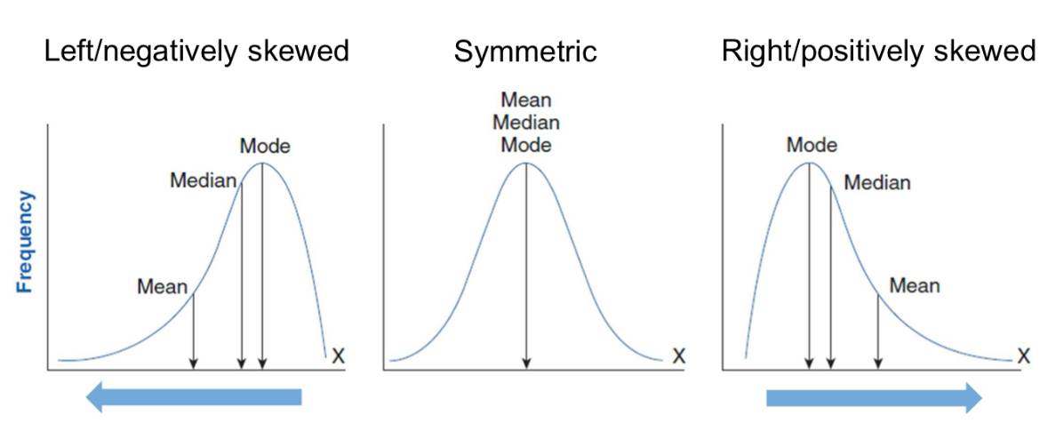
What are the three types of (skewed) distributions?

• Left (negative; mean < mode < median)

• Symmetric (mean=mode=median)

• Right (positive; mode > median > mean)

What are three measures of variability?

• Range (min. ordinal): x_max - x_min

• Interquartile range [IQR] (min. ordinal): Q_75% - Q_25% → shows how the middle 50% of the data varies

• Variance (min. interval): mean squared deviation from the average value (SD= sqr[s²]) → s²= (sum of [x_i - x_mean]² / n-1)

What are the two measures of the shape of a distribution?

• kurtosis (peakedness) → normal (0), peaked (positive), flattened (negative)

• skewness → symmetric (0), right-skewed (positive), left-skewed (negative)

What are the three ways to describe the association between two variables?

• Product-moment correlation (Pearson):

  • minimum interval scale

  • describes the strength and direction of a linear relationship between two continuous variables

  • r∈[−1,1]

    • r=1: Perfect positive linear relationship (as one variable increases, the other increases proportionally).

    • r=−1: Perfect negative linear relationship (as one variable increases, the other decreases proportionally).

    • r=0: No linear relationship.

  • very sensitive to outliers

• Rank correlation (Spearman):

  • minimum ordinal level

  • shows the strength and direction of a monotonic relationship (variables change in one direction) between two variables

  • uses ranks, not raw values

  • p∈[−1,1]

    • p=1: Perfect positive monotonic relationship (as one variable increases, the other always increases).

    • p=−1: Perfect negative monotonic relationship (as one variable increases, the other always decreases).

    • p=0: No monotonic relationship.

• Cramer’s V:

  • shows the strength of association between two categorical variables

  • nominal scale

  • r∈[0,1]

    • r= 1: Perfect association (categories completely dependent).

    • r=0: No association between variables.

    • cannot be negative because it measures strength, not direction

What is a scientific hypothesis?

• informed speculation about the possible relationship between two or more variables

• if (IV)… then (DV)… statements

What is a confounder variable?

• extraneous variable that has casual relationship to both the IV and the DV

• there is no direct causation between the IV and DV, they are connected by their correlation to the confounder variable

What is a mediator variable?

• an intervening variable that reflects the mechanism leading to the correlation between the IV and DV

• helps to understand the mechanism by which the IV and DV are associated

• conceptual, not easily measured

What is a moderator variable?

• affects the correlation between the IV and DV

• it isn’t caused by the IV, and it doesn’t cause the DV

What are the criteria for scientific hypotheses?

• Falsifiability: degree to which the hypothesis can be shown to be false

• Empirical content: number of ways in which a hypothesis can be falsified

  • Universality: how general is the “if” component

  • Precision: how specific is the “then” component?

  • the empirical content is high the more general and precise the hypothesis is

What is operationalization?

• translating abstract theoretical concepts into measurable variables

• defines how these concepts will be observed and quantified

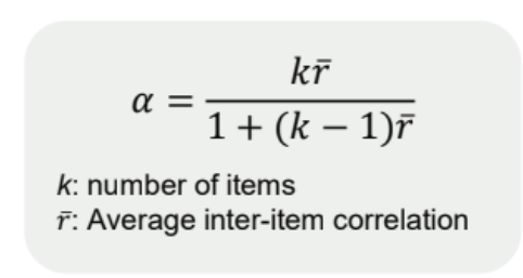
What is reliability, and what are its two types?

• consistency of the measurement when obtained by the same methodology on more than one occasion or across different but related test items

• Test-retest reliability: correlation of test scores across measurement occasions → is the measurement stable across time

• Internal reliability: are different items for measuring the construct consistent among themselves

  • Cronhach’s alpha → at lease .8

What is validity, and what are its four types?

• how well a measure or research design captures what it sets out to measure

• Convergent validity: high correlation of similar constructs

• Divergent validity: low correlation of unrelated constructs

• Internal validity: does the design allow for firm conclusions regarding the causal link between the DV and IV

• External validity: can the findings be generalized to settings outside the lab

What are the differences between correlational and experimental research?

• Correlational research: IV and DV vary naturally → can lead to confounder variable effects

• Experimental research: IV is manipulated to see how it affects the DV → participants are randomly allocated to different levels of IV

  • Between-subjects design: different people are presented with different levels

  • Within-subjects design: each person is presented with several levels

What is the quasi-experimental approach?

• the IV is manipulated, but the assignment to experimental vs. control group is not random

• assignment reduces confounder variables

• internal validity is lower, but external validity is higher

What is sampling error?

• difference between characteristics of the sample and of the population

• is smaller the larger the sample

What is probability sampling, and what are the three ways of doing it?

• any person in the population has a probability of being sampled

• Random: each person has the same chance

• Stratified random:

  • relevant characteristics are identified to form groups in the population

  • participants are randomly sampled from each group in proportion to their size in the population

  • ensures that the sample matches the population of these characteristics

• Cluster: relevant units of people are identified → some units are chosen to sample participants from them

What is non-probability sampling, and what are the four ways of doing it?

• some members of the population are systematically excluded from participation → leads to nonrepresentative sample

• Convenience: sampling participants that can be conveniently recruited

• Quota: subgroups are identified → specified number of individuals form each group are sampled by convenience

• Snowball: individual participants are sampled → identify participants from people they know

• Purposive (judgmental): participants are selected due to some desirable characteristics

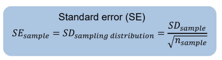
What is standard error and what does it show?

• tells how much the sample mean is expected to vary from the true population mean → variability of sample mean across repeated samples

• indicates the precision of the measurement

• decreases as sample size increases

What is the p-value?

• represents the probability of obtaining a test statistic at least as extreme as the one observed, assuming the null hypothesis is true

• indicates how “unusual” the observed value is under the null hypothesis

What is the Fisherian approach to hypothesis testing?

1. Set up a null hypothesis

2. Set up the probability distribution of results expected under the null hypothesis

3. Significance testing: determine p-value for obtained results

What is the Neyman-Pearson approach to hypothesis testing?

1. Set up the probability distributions for two hypotheses (H₀, H₁) → difference indicates the expected effect size

2. Identify Type I and Type II errors (α and β, respectively)

3. Set α and β before data collection (e.g., α = .05, β = .2)

4. Use α criterion for making a decision → desired level of Type I error

5. Calculate statistical power (1-β [=.8])

What is the process of null hypothesis significance testing?

1. Set up a null hypothesis

2. p-value: Probability of the observed test statistic (e.g., t, χ2, F) under the H₀ → p(data|H₀)

3. Report the exact p-value

4. Predefined level of Type I error, α (most commonly α = .05 or α = .01) → Reject H₀ if p-value ≤ α; do not reject H₀ if p-value > α

5. Effect size: (Normalized) difference between H0 and H1

6. Statistical power, 1-β (most commonly set to 1-β = .8)

What is the difference between one-tailed and two-tailed t-test?

• One-tailed: directional hypothesis

  • entire α is placed in one tail (e.g. 0.05) of the t-distribution

  • if the t-value falls in that tail, reject H₀

• Two-tailed: effect in either direction

  • α split across both tails (e.g. 0.025 each tail)

  • if the t-value is extreme in either tail, reject H₀

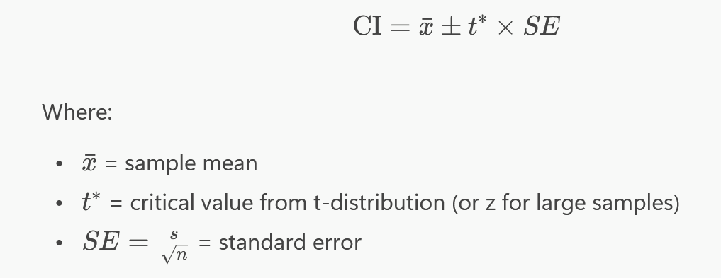
What is a confidence interval?

• range of values that is likely to contain the true population parameter with a specified level of confidence

• range of candidate population means that would not be rejected by a two-sided significance test

What is statistical power? What factors influence it?

• probability that a statistical test will detect an effect when the effect truly exist

• ideal 1-β > 0.8 → 80% chance to find a hypothetized effect if it’s true

• effects

  • sample size

    • larger sample → greater distribution → H₀ and H₁ graphs further apart

  • mean

  • α > 0.05 (falsely rejecting H₀)

  • small variance → greater power

What is a t-value, and what does it show?

• measures the difference between the sample data and H₀ in units of standard error

• larger t-value → likely reject the null hypothesis (t_crit > t_observed)

• Degrees of freedom: shows how much information is available for estimating variability

  • df= n₁ + n₂ - 2

What does Cohen’s d show?

• magnitude of the difference between two group means, expressed in standard deviation units

• measures the effect size → practical significance

• independent of sample size

• 0.2 → small effect, 0.5 → medium effect, 0.8 → large effect

What are the three types of t-test?

• Independent samples t-test: compare means of two independent groups

• Dependent samples t-test: compare means of two related observations (often within-subject design)

• One-sample t-test: comparing the mean of one group against a single value

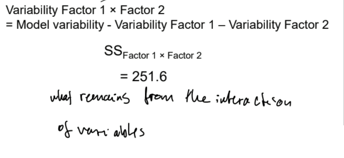
What is total variability?

shows how much the data points differ from the overall mean

total variability = model variability + residual variability

What is model variability?

• how much of the total variability is accounted for by the regression model or group differences → goodness of fit

• cells: combination of a unit of Factor 1 and Factor 2

What is residual variability?

• variability not explained by the model (error term/noise)

• cannot be explained by IV

What are variability factors?

• IVs that account for differences in the DV

• sources of variation in the data

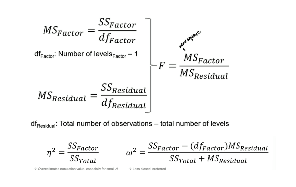
What does ANOVA show?

• tests how 3 or more groups means differ

• compares variability between groups to variability within groups

• F-statistic: ratio of explained variance to unexplained variance

  • large F-value (>1) → at least one group mean differs → model explains more variance than error

  • can only do one-tailed test

• Effect size: proportion of variance in DV explained by the IV → practical significance (what % of variation is due to the variables chosen)

  • .01 → small effect, .06 → medium effect, .14 → large effect

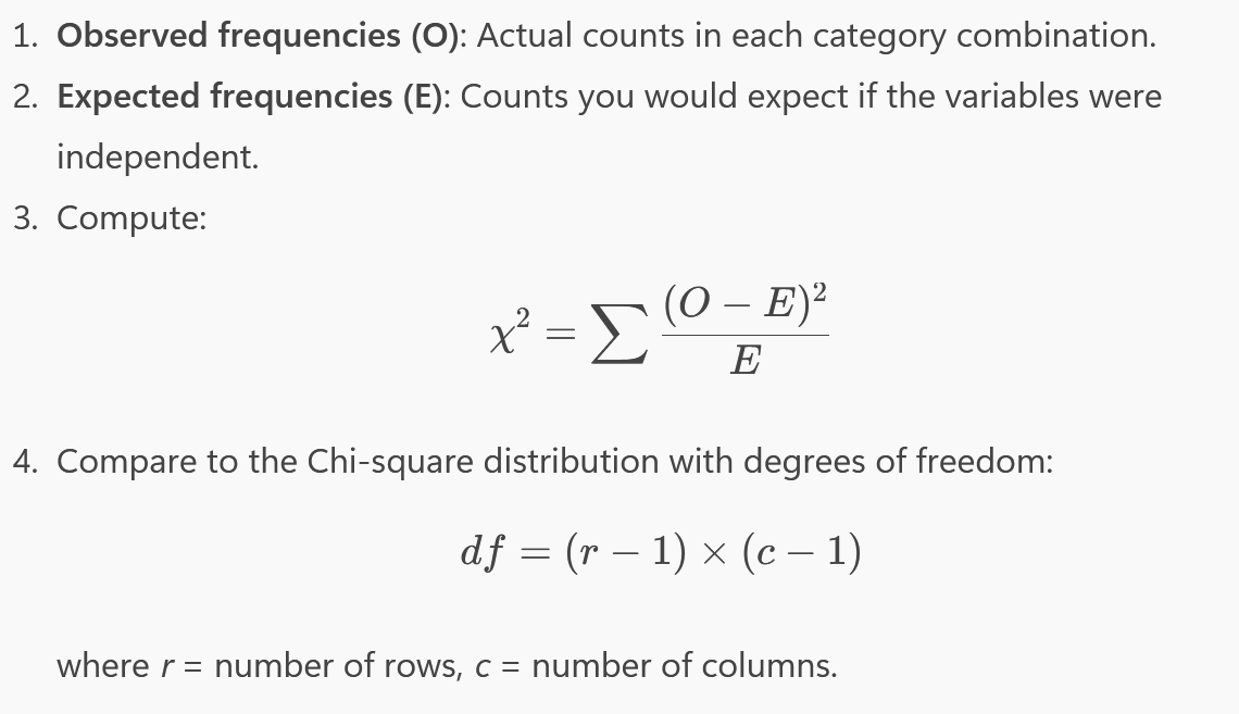
What does the Chi-square test show?

• examines whether there is an association between two categorical variables

• compares observed frequencies with expected frequencies (no association)

• significant result → one variable depends on the other

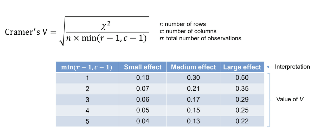
What is Cramer’s V?

Tells how strong the association is between the variables → effect size for Chi-square

What are the goals of regression analysis?

• describe a relationship between a DV and a predictor in a given set of observations

• predict the DV from a predictor for a new set of observations

What does it mean when a value is centered?

• shows how far the value is from the mean → facilitates interpretation of the intercept

• X_centered = X - X_mean

What is the purpose of the method of least squares (ordinary least squares)?

• minimizes the sum of squared differences between observed and predicted values

• squaring residuals → all differences positive → no cancellation

• gives line of best fit

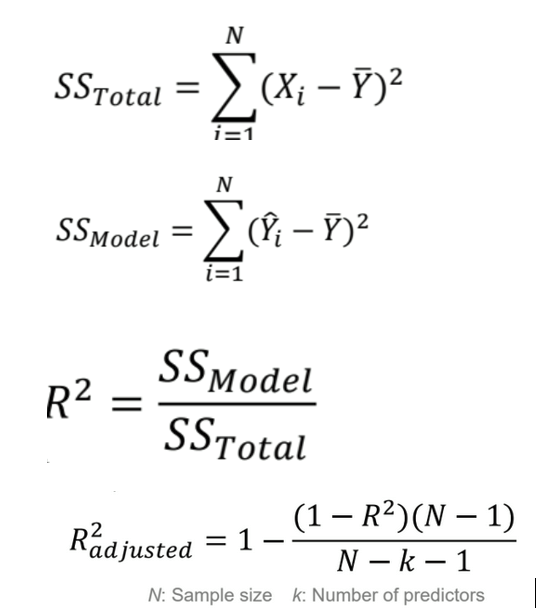
What does R² represent?

• measures the proportion of variance in the DV explained by the IV

• 0 → poor fit, 1 → model explains all variance

How is the regression coefficient b evaluated?

• test whether it is significantly different from 0

1. estimate using MLS

2. calculate standard error

3. compute 2-tailed t-statistic (only to positive side)

4. check p-value (b has no effect)

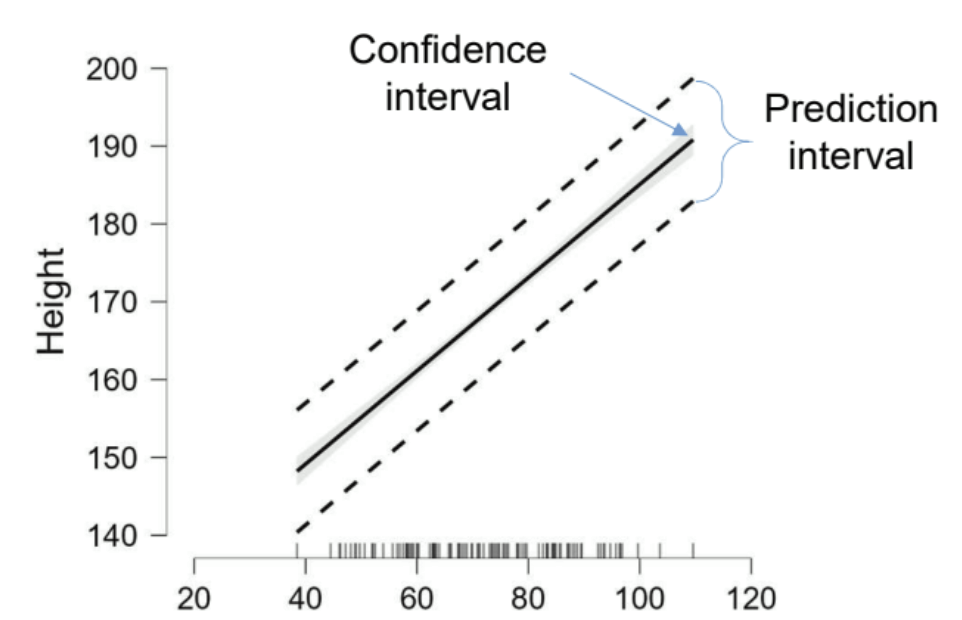
What is the confidence and prediction interval showing?

• Confidence interval: range within the average predicted value Y is likely to fall

  • precision of the estimate average Y for a given X

• Prediction interval: range within an individual observation of Y is likely to fall

  • wider than confidence interval because individuals vary more than the mean

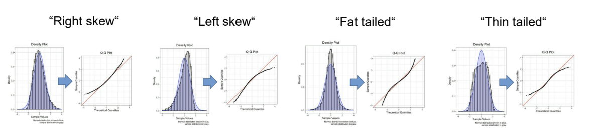
What three assumptions are made in regression analysis?

• Linearity

  • is the average value of the residuals similar across different levels of the predictor

• Homoscedasticity: at each level of the predictor variable, the variance of the residuals is the same

  • is the variability of the residuals similar across different levels of the predictor

• Normal distribution of residuals

  • Q-Q plot: expresses how many values in the distribution are below a certain value

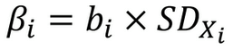
In a multiple regression, why do coefficients need to be standardized?

• allows for comparison of regression coefficients between predictors

• standardized coefficients show changes in terms of standard deviations

Compared to linear regression, what extra assumption needs to be made for multiple regression?

Absence of multicollinearity: correlations among predictors should not be too large (r < .8)

How can multicollinearity be evaluated for?

• check intercorrelations among predictors

• Tolerance: degree to which a given predictor can be predicted by the other predictors

  • 1-R_x² → higher, the better

  • 0.1 → 90% of variance of one is within the other set

• Variance inflation factor (VIF): 1/tolerance

  • largest should not be greater than 10

  • average should not be much greater than 1

• if multicollinearity present

  • drop redundant predictors

  • combine highly correlated predictors with factor analysis

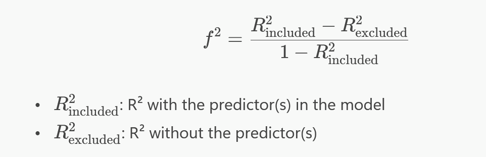
What does effect size f² show in multiple regression?

• quantifies the impact of a predictor on the DV beyond what is already explained by other predictors

• .02 → small effect, .15 → medium effect, .35 → large effect

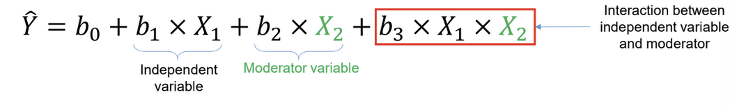
What is moderation analysis?

• checks if the effect of the IV on the DV differ between categories of the moderator variable

  • e.g. weight (IV) and height (DV) in males and females (MV)

• tested by including the IV, the moderator, and their interaction as predictors

  • regression coefficient of the interaction is obtained by subtracting the coefficients of each MV from each other

What is mediation analysis?

• three conditions

  • significant relationship between IV and DV

  • significant relationship between IV and mediator

  • significant relationship between mediator and DV, controlling for the IV

• shows if the path from IV to DV is reduced when mediator and IV are used simultaneously to predict the DV → is the indirect effect reliably different from zero

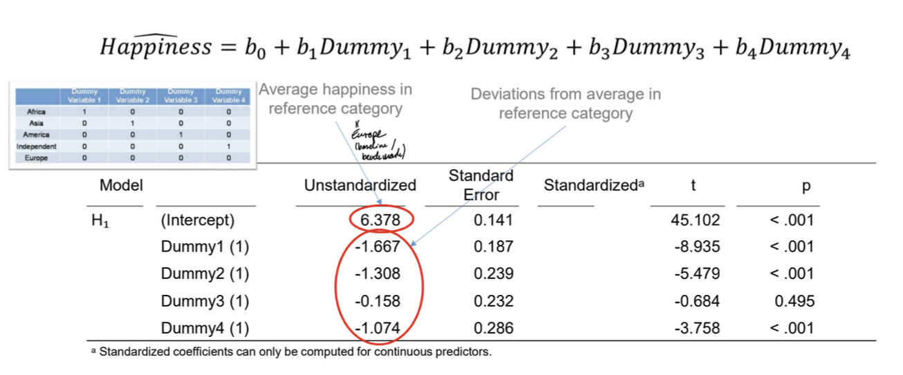
What is the purpose of dummy coding?

• construct multiple regression for categorical predictors

• procedure

  • k categories → k-1 dummy variables

  • set reference category (to which all are compared) to 0 → each dummy variable is a combination of 1 and all others 0

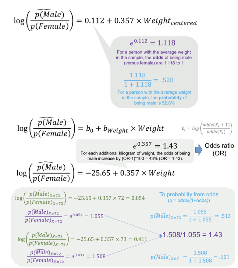
What is the general formula for probability and log odds?

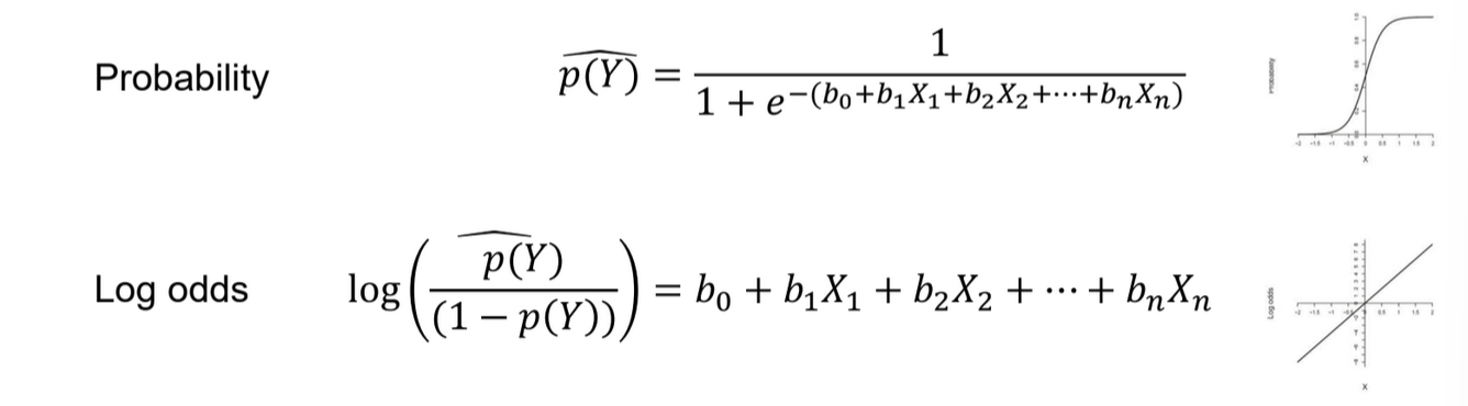
What is the relationship between probability, odds, and log odds?

• Probability: likelihood of an event occurring

• Odds: ratio of the probability of an event occurring to the probability of it not occurring

• Log odds: log of odds → linear scale

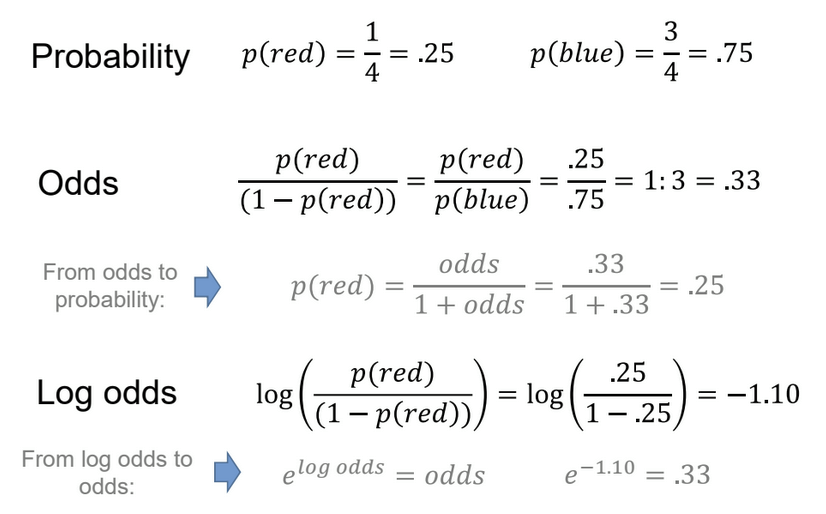
How to interpret the logit function values

odds ratio is always constant

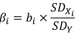
What does the standardized regression coefficient show?

• how strongly a predictor variable influences the DV in standard deviation units → allows for comparison across continuous predictors

• “how many standard deviation units Y changes when X increases by one unit of standard deviation”

• not for nominal and binary values

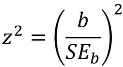
What does the Wald statistic show?

• tests whether a regression coefficient is significantly different from zero

• 0 → predictor is non-significant

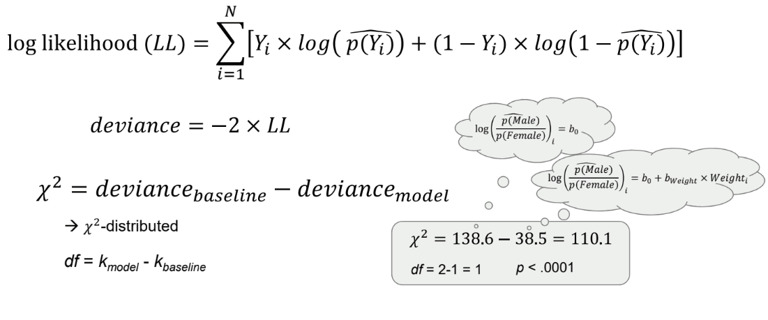
What is log likelihood and deviance?

• Log likelihood: measures how well the statistical model explains the observed data

  • smaller → worse fit of model

  • used for AIC and BIC calculation

• Deviance: measures how far a model is from the “perfect” model

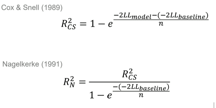
How do the Cox & Snell and Nagelkerke models differ?

• both measure pseudo-R² (no real R² in logistic regression)

• Cox & Snell:

  • Mimics linear regression R² as closely as possible

  • % of log likelihood variation

  • never reaches 1, even for a perfect model → bounded below 1

• Nagelkerke:

  • adjusted version of Cox & Snell → can reach 1

  • % of maximum possible improvement

What is a confusion matrix?

• a table that shows how well the model predicts categories

• compares predicted and actual classes → % of correct predictions

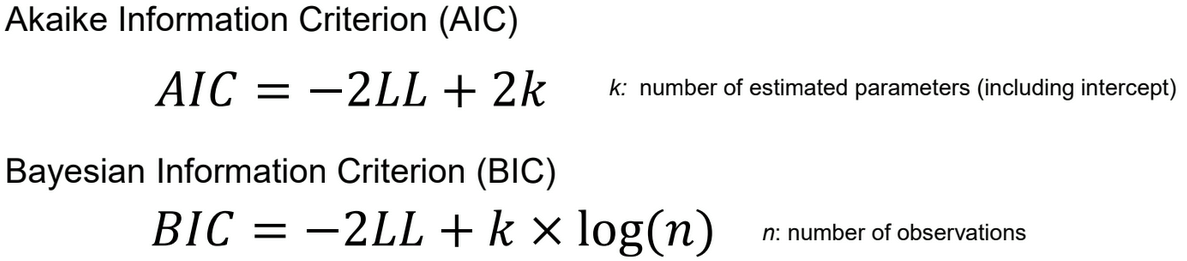
What does AIC and BIC show?

• how well a model fits the data while penalizing for model complexity

• low values → better trade-off between model fit and model complexity

• AIC → accounts for how simple the model is

• BIC → stronger penalty for complexity

What are the three important requirements in logistic regression?

• absence of multicollinearity

• linearity (in log-odds space)

• no complete separation of data between two categories

What is the sample-size consideration for logistic regression?

At least 10 events per predictor (cases in less frequent category of DV)

What are the goals of factor-analytic techniques?

• discover factors responsible for covariation among multiple observed variables

• reduce a large set of variables into a smaller set of factors

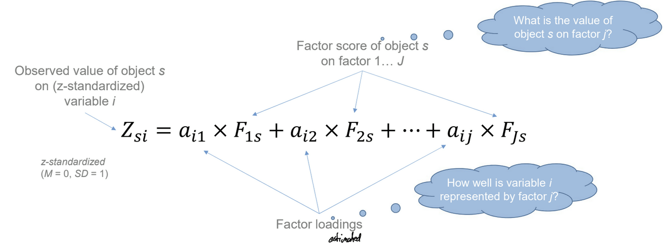
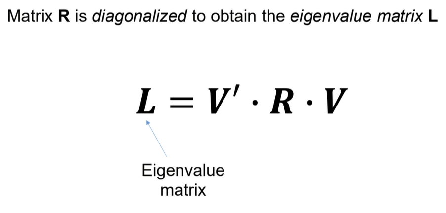
What is principal component analysis, and how is it calculated?

• PCA finds patterns in how variables co-vary and summarizes them → new variables represent the main directions of variation

• calculation

1. z-standardize variables

2. correlation matrix

3. calculate eigenvalues

4. determine how many components to keep

5. compute factor loadings

6. (rotate components)

7. compute factor scores

What is an eigenvalue?

• explains how much of the total variation in the data is captured by each component = how much variance is being explained by the factors being extracted

• large value → important component

• uses values coming from the correlation matrix (Pearson’s coefficients comparing two components at a time)

• can also be obtained as the sum of factor loadings for each PC (column-wise)

What are the three ways it can be calculated how many factors should be retained in factor analysis?

• Scree test: eigenvalues are plotted in descending order → Elbow Criterion: cutoff where the distribution of eigenvalues levels off

• Kaiser criterion: retain components with an eigenvalue > 1

• Parallel analysis: benchmark based on comparing observed eigenvalues with random data → cutoff where graph of observed gets below graph of predicted

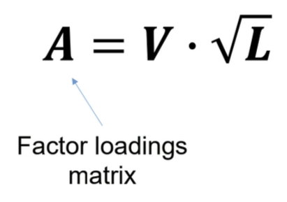
What is a factor loadings matrix? What do communality and uniqueness describe?

• explains how much each variable contributes to a factor

• each cell shows the correlation between an observed variable and a latent factor → factor loading

• > .4 → high, < .2 → low, negative → opposite correlation

• commonality:

  • proportion of variance explained by the factors

  • sum of PC values for each item (row-wise)

• uniqueness:

  • proportion of variance not accounted for by the factors

  • 1 - communality

What is the purpose of rotating factor loadings?

• high loading values on multiple factors for multiple items → simplification of structure needed

• considers correlation between variables as angles between vectors

  • small angle → high correlation

  • more than 90° → negative correlation

  • correlation (r): cosine of the angle between two vectors

What are the four ways to rotate factor loadings?

• Orthogonal

  • Varimax: maximize variance of squared factor loadings across variables → allocates each variable to one factor → very high or very low values for each factor → multiple distinct factors

  • Quartimax: maximize variance of squared factor loadings across factors → creates one general factor most variables load on → simplifies factors, not variables → one general underlying factor

• Oblique

  • Oblimin: minimize cross-products (overlap) of loadings → less extreme values than Promax

  • Promax: based on varimax but with “flexibility” → cleaner results, more tolerant of messy data

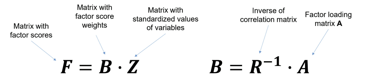
What are factor scores?

Values of the objects for each factor

What are preparatory considerations for a PCA?

• interval scale

• normal distribution

• intercorrelation matrix mostly with values .3 or higher → little covariation

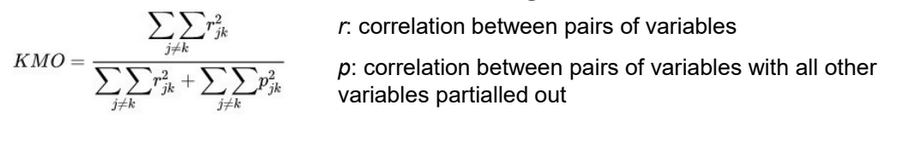
• Bartlett’s test of sphericity:

  • tests whether there is enough correlation between the variables to justify running a factor analysis

  • see whether the variance-covariance matrix is not an identity matrix → refute null hypothesis

• Kaiser-Meyer-Olkin (KMO) measure of sampling adequacy (> .6)

  • quantifies whether there is shared variance among the variables

  • tests not only presence of correlation, but strength

What two factors should be taken into consideration when planning the sample size for PCA?

• at least 10 objects per variable

• at least 4 variables per factor

• parameters become stable with about 300 objects

• (if communalities are > .6 → clear structuring of data → small number of objects sufficient)

What is the goal of cluster analysis?

Find clusters within which objects are as similar as possible (internal homogeneity), while at the same time, between clusters the objects are as distinct from each other as possible (external heterogeneity)

What is the general procedure of cluster analysis?

1. Quantify similarity of objects

2. Group objects into clusters according to similarity

3. Determine the optimal number of clusters (complexity vs. model fit)

4. Interpret obtained clusters

What are the two ways to quantify similarity?

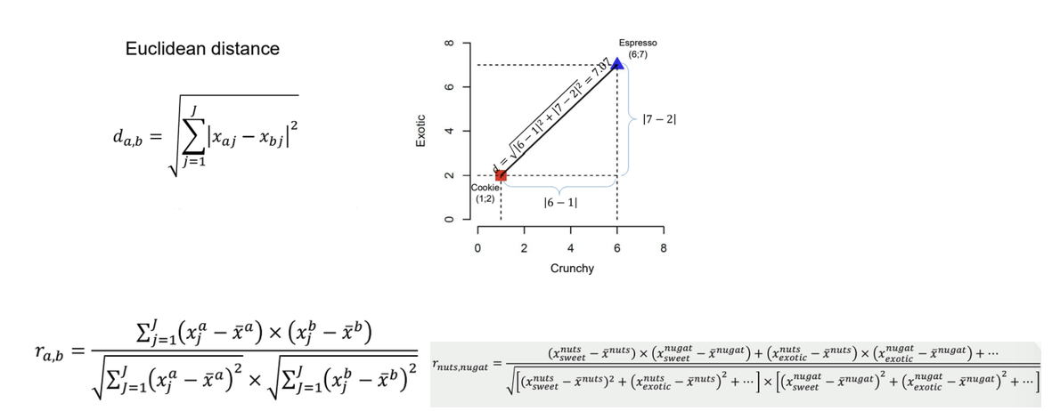
• Euclidean distance: calculate distance based on the position of the values in a graph

  • higher values of d → lower similarity

• Correlation: checks if two variables have similar patterns of variation across different variables

  • higher r → higher similarity, negative → correlation in opposite direction

What are the two ways hierarchical clustering can be done?

• agglomerative: start from each object as a separate cluster, then reduce the number of clusters

  1. calculate pairwise similarity between objects (distance or correlation)

  2. merge objects with highest similarity into a cluster

  3. calculate linkage criterion for new candidate clusters → ranking

  4. choose candidate cluster that minimizes linkage criterion

  5. repeat step 3 & 4 until there is a single cluster

• divisive: start from one cluster

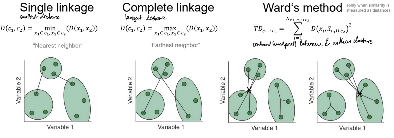
What are the three linkage methods?

• Single linkage: looks at closest pair of points → clusters if objects are close

• Complete linkage: looks at farthest pair of points → cluster objects together that are far from another cluster

• Ward’s method: minimize total distance of objects within a new candidate cluster → compares distance of objects from the centroid (average) of a cluster

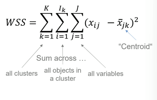
What does the within-cluster sum of squares show?

WSS measures model fit → takes deviation from centroid for each cluster → more clusters = lower WSS

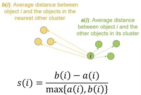
What is the Silhouette coefficient?

• indicates how clearly clusters are separated

  • measures how similar an object is to its own cluster (cohesion) relative to other clusters (separation)

  • -1 → overlapping clusters, +1 → homogeneity within cluster, distinction from neighboring cluster

  • high values → appropriate clustering

What is the goal and principle of conjoint analysis?

• preference is based on a combination of all attributes (CONsidered JOINTly)

• Goal: determine how important different attributes and attribute levels are for people’s preferences → decompositional method

• Principle: create options as a combination of different attribute levels, then measure people’s preferences for the different options → infer impact of attributes and attribute levels

What are the general steps of a conjoint analysis?

1. Selection of attributes and attribute levels

2. Design of the options + collection of preferences

3. Parthworth utilities

4. Importance of individual attributes

What are the six criteria for selecting attributes and attribute levels?

• Relevance: attributes must be relevant for people’s preferences

• Actionable attributes: attributes should be modifiable

• Realistic and feasible: the attribute levels and their combinations should be plausible

• Manageable number of attributes and attribute levels: the number of attributes and attribute levels should not be too high

• Compensatoriness: the attributes should be able to compensate each other → no exclusion criteria

• Independence: the utility of an attribute level should not depend on the value of another attribute

What is the difference between a full and a fractional orthogonal design?

• Full: all possible designs are listed

• Fractional: get a smaller set of combinations where attributes are still uncorrelated → based on simulation methods