Stats Midterm 2 REVIEW

Tafeshi- Ch.11 and 12, Lane- Ch.9 and 11

true or false there is sampling distribution for various of sample sizes

true

Mean

µM = µ

-mean of sampling distribution is the mean of the poplulation we sampled

Um-mean of the sampling distribition

Variance

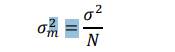
-variance of sampling distribition of the mean is the population variance divided by N, sample size

-larger sample size,the smaller the variance of the sampling distribution of the mean

proability value

proability of an outcome, and not the proablity of a particular state of the world

Null Hypothesis

Null hypothesis is the opposite of the reasercher hypothesis

-the null hypothesis are two types of patients are treated identically with the hope one can be discredited and therfore rejected

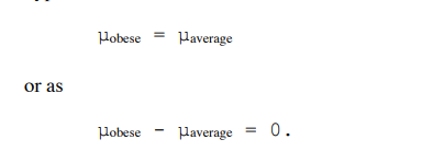
If the null hypothesis is rejected, then the alternative to the null hypothesis (called the alternative hypothesis) is accepted. The alternative hypothesis is simply the reverse of the null hypothesis. If the null hypothesis µobese = µaverage is rejected, then there are two alternatives: µobese < µaverage µobese > µaverage.

steps in hypothesis testing

1. The first step is to specify the null hypothesis. For a two-tailed test, the null hypothesis is typically that a parameter equals zero although there are exceptions. A typical null hypothesis is μ1 - μ2 = 0 which is equivalent to μ1 = μ2. For a one-tailed test, the null hypothesis is either that a parameter is greater than or equal to zero or that a parameter is less than or equal to zero. If the prediction is that μ1 is larger than μ2, then the null hypothesis (the reverse of the prediction) is μ2 - μ1 ≥ 0. This is equivalent to μ1 ≤ μ2.’

2. The second step is to specify the α level which is also known as the significance level. Typical values are 0.05 and 0.01.

3. The third step is to compute the probability value (also known as the p value). This is the probability of obtaining a sample statistic as different or more different from the parameter specified in the null hypothesis given that the null hypothesis is true.

4. Finally, compare the probability value with the α level. If the probability value is lower then you reject the null hypothesis. Keep in mind that rejecting the null hypothesis is not an all-or-none decision. The lower the probability value, the more confidence you can have that the null hypothesis is false. However, if your probability value is higher than the conventional α level of 0.05, most scientists will consider your findings inconclusive. Failure to reject the null hypothesis does not constitute support for the null hypothesis. It just means you do not have sufficiently strong data to reject it.

Misconceptions of signifiance testing

Misconception: The probability value is the probability that the null hypothesis is false. Proper interpretation: The probability value is the probability of a result as extreme or more extreme given that the null hypothesis is true. It is the probability of the data given the null hypothesis. It is not the probability that the null hypothesis is false.

2. Misconception: A low probability value indicates a large effect. Proper interpretation: A low probability value indicates that the sample outcome (or one more extreme) would be very unlikely if the null hypothesis were true. A low probability value can occur with small effect sizes, particularly if the sample size is large.

3. Misconception: A non-significant outcome means that the null hypothesis is probably true. Proper interpretation: A non-significant outcome means that the data do not conclusively demonstrate that the null hypothesis is false.

why do experiementers test hypotheses they think are false?

Providing data that supports a hypothesis does not mean that it is true, just that there is no evidence that contradicts it. Providing evidence that is contrary to a hypothesis allows you to reject that hypothesis as false.

difference between proablity value and signifiance level?

Proablity Value: -Measures the strength of the evidence against the null hypothesis

The actual calculated probability of finding your observed or more extreme data under the assumption of pure chance

-Calculated after you collect your data and perform your statistical test.

Signifiance level:

The maximum probability threshold you are willing to accept of incorrectly rejecting the null hypothesis (a Type I error).

Set before the data is collected or analyzed to avoid bias (usually set to 0.05 or 0.01).

True/false: You are more likely to make a Type I error when using a small sample than when using a large sample.

false

True/false: You accept the alternative hypothesis when you reject the null hypothesis.

true

True/false: You do not accept the null hypothesis when you fail to reject it.

true

True/false: A researcher risks making a Type I error any time the null hypothesis is rejected.

true

True/false: The standard error of the mean is smaller when N = 20 than when N = 10.

true

True/false: The sampling distribution of r = .8 becomes normal as N increases.

false

True/false: You choose 20 students from the population and calculate the mean of their test scores. You repeat this process 100 times and plot the distribution of the means. In this case, the sample size is 100.

false

True/false: In your school, 40% of students watch TV at night. You randomly ask 5 students every day if they watch TV at night. Every day, you would find that 2 of the 5 do watch TV at night.

false

True/false: The median has a sampling distribution.

true

Population parameters

based on stattiscs calculated on samples of raw data

random sampling

drawing our sample from our population of interest

-random sampling that the process by which objects/events are drawn from our population is random

simple random sampling

-is a random sampling technique in which every element belonging to an object/event that is drwan from our population always has an equal and consistent proablility of being drwan

sampling error

every time I draw a random sample from the population, I will end up with a different sample mean

any population with a µ and σ2

𝜇"# = µ. The mean of a sampling distribution of the mean (i.e., the expected value) is equal to the mean of the population from which the sample means are derived. This means that the expected value is an unbiased estimator of the population mean.

2. 𝜎"# $ = %# & and 𝜎𝑋I = 𝜎 √𝑁 . The variance of the sampling distribution of the mean for a given sample size is equal to the variance of the parent population divided by the sample size. The standard deviation (i.e., standard error) of the sampling distribution of the mean for a given sample size is equal to the standard deviation of the parent population divided by the square root of the sample size.

3. As N reaches infinity, the sampling distribution of the mean will increasingly approximate, or, if the parent population is normal in shape, will be, a normal distribution. This means that the sampling distribution of the mean derived from a normal parent population will be normal in shape. It also means that regardless of what shape your parent population is, as N increases, the sampling distribution of the mean will approach a normal distribution.

what is the importance of random sampling?

ensures that every single member of population has an equal independent chance of being selected for the study

1. elimations selection bias

2. creates representitive sample

3. satisfies assumptions of statisical tests

4. simplifies data analysis

what is sampling problem?

the challenge of selecting a small subset of individuals from a larger population that accurately represents the whloe group

-selection bias and sampling error

Describe two ways that sample size has an impact on the sampling distribution of the mean.

-sample size increases the standard error gets smaller

-A larger sample size pulls the sample means tighter around the true population mean. It reduces variability from one sample to the next, making your statistical estimates much more precise and reliable.

Even if your underlying population data is heavily skewed, bi-modal, or completely uniform, a large sample size smooths out those irregularities. This allows researchers to safely use parametric statistical tests (like t-tests and Z-tests) that strictly require normally distributed data.

Step 1 of null hypothesis testing

-state the population distribition of the ramdom variables of interest

-when makinmg statisical inferences, we don’t actually know what to expect from the population of interest

-it is hard for us to be able to infer whether our sample is truly representative of the population

what the form of the theoretical population distribution of a random variable of interest is

𝑋 ~ 𝑁(𝜇, 𝜎%)

step 2 of null hypothesis testing

-state the null and alternative hypothesis

-parmeter of interest

-involves stating a null hypothesis and alternative

-do not confuse these with the research hypothesis

-testeable formulations of what the researcher expects from the parameters of interest

-Retain Ho or reject Ho

null hypothesis

will state what is expected from the given parameter of interest when there is no interesting “effect

-HO retain or reject Ho

alternative hypothesis

will state what is expected from the given parameter of interest when there is no interesting “effect

Non-directional hypothesis

Because the researcher is interested in deviations from the average score in either direction (above or below

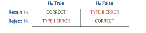
type I error

to the instance in which the researcher rejects the null hypothesis when it is actually true in nature

The long-run probability of making a type I error is referred to as alpha (α). This is sometimes called the “type I error rate”. Alpha is a value that is specified by the researcher (usually at a small value) and exists under the null distribution (the distribution implied by the null hypothesis)

type II error

to the instance in which the researcher accepts the null hypothesis when it is actually false in nature

The long-run probability of making a type II error is referred to as beta (β), or the “type II error rate”. Unlike alpha, beta exists under an alternative distribution. This means that it exists under a distribution that is implied by one of a number of alternative distributions that might actually be the case in nature

step 3 (null hypothesis testing)

-state the assumptions of the test

By asserting a particular form of the distribution of the parent population, we are also making several assumptions about its distribution.

step 4 (null hypothesis testing)

is means that there will be at least one statistic calculated on our raw data that will be used to make inferences about the population. This statistic is often referred to as our observed statistic or test statistic (denoted as statobs).

1. The expected value of the sampling distribution of the mean is equal to the population mean.

2. The sampling distribution of the mean gives us the probabilities associated with obtaining (roughly) a particular value of the mean.

Given this information, we know that we simply need to compare our sample mean to the sampling distribution of the mean under the condition that H0 is true, or what is often referred to as the null distribution in a NHST scenario, to determine how likely it is that our sample mean is in keeping with the sampling distribution (aka null distribution) implied by our null hypothesis

If the null hypothesis is true, and the assumptions are true, then our test statistic will have a particular theoretical distribution (this is the “null distribution”).

step 5- specify alpha and decision rule

Specifically, we need to say how much our test statistic needs to deviate from the mean of the null distribution for us to say that our sample is not likely to be derived from the specified null distribution. We do this by specifying the size of the probability under the null distribution associated with obtaining a value as or more extreme than our test statistic that would be small enough for us to conclude that the test statistic is not from the null distribution. This probability is called alpha (𝛼) – it’s also our Type I Error rate.

critical value or statcrit

hen we are dealing with a specified theoretical distribution, such as the standard normal, we often specify the test statistic as zobs and the critical value as zcrit.

hen we are dealing with a specified theoretical distribution, such as the standard normal, we often specify the test statistic as zobs and the critical value as zcrit.

one tailed test

-only haave one critical value that fell on one tail of the distribution

two-tailed test

-when testing non-directional hypothesis, we are interested in scores deviating from the mean in either direction

decision rule

If pobs < 𝛼, then reject H0; otherwise, retain H0.

Since our critical values are tied to our specification of 𝛼, an alternative, equivalent, decision rule is: If statobs is more extreme than statcrit, reject H0; otherwise retain H0\

What is meant by “more extreme” is that statobs falls further out into the tail end(s) of the distribution than statcrit. How many and which end will depend on your hypotheses. These 2 decision rules are equivalent and will give the exact same result.

Notice the relationship between pobs and statobs for standard normal distributions

: As |statobs| à ∞, pobs à 0

As |statobs| à 0, pobs à 1

step 6

-conduct the study, calculate desripitive statisics and check on assumptions

-This stage of the process involves designing and implementing your research study (i.e., data collection) – similar to what you will do in your research methods class. We won’t be collecting any actual data in the current class, but note that this is the stage at which you would actually do so.

Once we have our data, we can display it and calculate descriptive statistics (conduct data analysis). At this point, we will also want to check on our assumptions. For example, if one of our assumptions is normality of the distribution, we can use graphical aids (e.g., a histogram) to plot our data to check that the normality assumption for the population appears to be sound. We can also check our g1 and g2 statistics to see how symmetric and mesokurtic our distribution is.

step 7 of null hypothesis testing

-run test and make decision

-we calculate our test statistic and identify the probability of obtaining a value as or more extreme than our test statistic under the null distribution (pobs). Once we have pobs we can compare it with our pre-specified alpha (or, alternatively, we could Intro to Statistics | ©Donna Tafreshi 2016 |172 compare our test statistic (statobs) with our critical value(s) (statcrit)) in order to make a decision.

Importantly, if you do end up rejecting the null hypothesis, you should compute an effect size to determine how large the effect that you have observed is and whether it is of practical value. Essentially, the idea here is that you have determined that there is a “statistically significant” result, and thus, that there is some sort of “effect” in your findings, or some departure of the actual value of the parameter of interest from the value of the parameter specified under the null hypothesis. How this is computed, and whether it is standardized or unstandardized, will vary across tests and purposes. I’ll provide some common effect size estimates as we go through various hypothesis testing scenarios in the remainder of the course

confidence intervals (CIs)

interval estimamtes of parameters

true or falase the bounds or limits that sit on either end of a confidence interval is confidence limit and there is upper confidence limit and lower confidence limit

true

formula for confidence limit (upper and lower)

𝑈𝐶𝐿 = 𝑋 + |𝑠𝑡𝑎𝑡BL!M| ∗ 𝑆𝐸

𝐿𝐶𝐿 = 𝑋 − |𝑠𝑡𝑎𝑡BL!M| ∗ 𝑆𝐸

third rule for hypothesis testing

if the confidence interval built around the sample mean captures the value of 𝜇 asserted by the null hypothesis, retain H0; otherwise, reject H0.

Describe how null hypothesis statistical testing offers a solution to the sampling problem.

NHST-solves the sampling problem

-sampling error may be a result due to small sample size

How NHST solves it:

1. creating a no effect (if null hypothesis Ho

2. models random chance

3. calculates the proablity score (p-value)

4. applies on objective cutoff (alpha level)

Describe the difference between a one-tailed and two-tailed test and explain how you know if your test is one-tailed or two-tailed.

-directionality of the alternative hypothesis (H1)

-one tailed test looks for change in specfic direction, and two tailed test looks for any change regardless of the direction

one tailed test-

Splits your entire critical alpha risk region (usually \(5\%\)) into a single tail of the probability distribution. It tests whether a sample value is significantly greater than or significantly less than a value, but not both.

for exmaple increase, lower, and reduce

two tailed test-

plits your critical alpha risk region equally into two halves (e.g., \(2.5\%\) in the left tail, \(2.5\%\) in the right tail). It tests whether a sample value is simply different from a baseline value, capturing changes in either direction.

for exmaple affect, difference and chnage

A population of scores has σ = 20. For random samples of n = 25, what is the standard error of the mean σX¯ = σ √ n ?

4

A population has σ = 15. Samples of size n = 9 are drawn. Compute σX¯ .

5

If σ = 12 and n = 36, what is σX¯ ?

12

Using the textbook example from lecture: textbooks have µ = 2.0 lbs and σ = 0.3 lbs. For a sample of n = 9 books, what is σX

0.1 Ibs

Using the coffee-shop example: µ = 400 customers/day, σ = 80. For a sample of n = 16 stores, what is σX¯ ?

20

A population has σ = 10. Samples of n = 100 give which standard error of the mean?

1

If σ = 24 and n = 64, what is σX¯ ?

3

A population has σ = 6. For a sample of n = 50, what is σX¯ (to two decimals)

0.85

Textbook weights: µ = 2.0 lbs, σ = 0.3 lbs, n = 9. A sample yields X¯ = 2.15 lbs. Compute z = X¯ − µ σ/√ n .

1.50

Coffee-shop chain: µ = 400, σ = 80, n = 16. The regional manager’s sample has X¯ = 385. Compute the z for this sample mean.

-0.75

For an IQ-like population with µ = 100, σ = 15, a sample of n = 25 gives X¯ = 106. What is z?

2.00

A population has µ = 500, σ = 100. A sample of n = 25 has X¯ = 520. Compute z for X¯.

1.00

According to the deck, to cut the standard error of the mean in half, you must:

Quadruple the sample size

. If n is increased from 25 to 100 (holding σ fixed), the standard error of the mean is multiplied by:

1/2

A population has µ = 50, σ = 10. A sample of n = 4 has X¯ = 53. What is z?

0.60

. According to the Central Limit Theorem as presented in lecture, the distribution of sample means centers exactly on:

The population mean µ

The standard error of the mean is best described (per the lecture) as:

The standard deviation of all possible sample means

Why does the standard error of the mean shrink as n grows?

Because σX¯ = σ/√ n, so dividing by a larger √ n yields a smaller value

Which statement best describes when the standard error (rather than the standard deviation) should be reported, according to the coffee-shop worked example?

When describing how precise the sample mean is as an estimate of µ

In your own words, state what the Central Limit Theorem guarantees about the distribution of sample means, and explain why this is useful when we do not know µ.

CLT guarantees the sampling distribution of X¯ is approximately normal, centered on µ, with standard deviation σ/√ n. This lets us place a single sample mean on a known distribution and reason probabilistically about µ even though µ is hidden.

Explain the “statistical hierarchy” from the deck: individual → sample → population, and how standard error is the natural analogue of standard deviation one level up.

Individuals deviate from their sample mean (σ / s capture this one level up from the individual). Samples deviate from the population mean (σX¯ captures this one more level up). SEM applies the same “average squared deviation” logic, but to means rather than individuals.

State one key assumption the deck highlights for using CLT-based inference, and explain what it means for the estimate if the assumption is violated.

Key assumption: random sampling (and CLT’s distributional assumptions). If violated, the sampling distribution may not center on µ or may not be approximately normal, so probability statements based on σX¯ become unreliable; small SE no longer guarantees the estimate is near the truth

A publisher reports textbooks weigh µ = 2.0 lbs with σ = 0.3 lbs. A manager samples n = 9 books and gets X¯ = 2.15 lbs. (a) Compute σX¯ . (b) Compute the z for this sample mean. (c) Interpret what the standard error of 0.1 lbs means in plain language.

) σX¯ = 0.3/ √ 9 = 0.1 lbs. (b) z = (2.15 − 2.0)/0.1 = 1.50. (c) “If the manager repeatedly drew samples of 9 textbooks, the sample means would typically differ from µ = 2.0 lbs by about 0.1 lbs.

A coffee-shop chain has µ = 400 customers/day and σ = 80. A regional manager surveys n = 16 stores and finds X¯ = 385. (a) Should the manager report the standard deviation or the standard error to show how precise his estimate of 385 is? Justify. (b) Compute that number. (c) Compute the z for X¯ = 385 and briefly interpret it.

Standard error: he is describing the precision of the sample mean, not store-to-store spread. (b) σX¯ = 80/ √ 16 = 20. (c) z = (385 − 400)/20 = −0.75; the observed mean is three-quarters of one standard error below µ, well within typical sampling variation.

A researcher is planning a study from a population with σ = 30. Currently she plans n = 25. (a) Compute the current standard error of the mean. (b) What sample size would be needed to cut that standard error in half? (c) Explain, using the deck’s “Law of Diminishing Returns” idea, why doubling n (from 25 to 50) does not cut the standard error in half.

σX¯ = 30/ √ 25 = 6. (b) To halve SEM, √ n must double, so n must quadruple: n = 100. (c) Because SEM depends on √ n, not n; doubling n only multiplies √ n by √ 2 ≈ 1.41, so SEM drops by about 29%, not 50% — each added observation buys less precision than the last.

A researcher tests H0 : µ = 100 versus H1 : µ ̸= 100 at α = .05. With X¯ = 108, σ = 15, n = 25, the z-test statistic is:

2.67

For the study in Q1, using zcrit = ±1.96, the decision is:

Reject Ho

A clinic tests H0 : µ = 50 versus H1 : µ ̸= 50. Given X¯ = 46, σ = 10, n = 25, compute σX¯ and z:

σX¯ = 2.0, z = −2.00

Using the deck’s worked example, a z of −2.0 in a one-tailed (lower) test corresponds to a tail probability of approximately:

0.0228

. For a two-tailed test at α = .05, the critical z values that define the rejection region are:

±2.33

For a one-tailed test at α = .05 (upper tail), the critical z value is:

+1.645

For a two-tailed test at α = .01, the critical z values are:

±2.58

For a one-tailed test at α = .01 (upper tail), the critical z is:

+2.33

A sample of n = 100 students yields X¯ = 105 when H0 : µ = 100, σ = 20. The z-test statistic is:

2.50

or the study in Q9 tested two-tailed at α = .05 (zcrit = ±1.96), the correct decision is:

Reject H0

Given H0 : µ = 30, X¯ = 26, σ = 12, n = 64, the z-statistic is:

-2.67

Using the deck’s rule that a z of 1.80 is “significant one-tailed but not two-tailed” at α = .05, which statement is correct?

|1.80| > 1.645 but |1.80| < 1.96

H0 : µ = 150, X¯ = 155, σ = 30, n = 144. The z-statistic is:

2.00

Using the deck’s worked example (X¯ = 46, µ0 = 50, σX¯ = 2, z = −2.0, one-tailed p = 0.0228) with α = .05, the correct decision and interpretation is:

Reject H0; p < α, the sample is too rare under H0

the p-value is best defined as:

P(data at least as extreme as observed | H0 true)

Why do we use a null hypothesis at all

Because inference is “one-way”—we cannot prove a universal truth, but we can disprove a lie

“Statistical significance” at α = .05, according to the deck, means:

The observed result is rare enough under H0 that we reject H0 as a plausible explanation

A Type I error occurs when we:

Reject H0 when H0 is actually true

A Type II error occurs when we:

Fail to reject H0 when H0 is actually false

Statistical power is best expressed as

1 − β

Per Popper’s logic (deck), which of the following is true about H0?

H0 can be rejected (falsified) but never proven true—only provisionally retained

State, in symbols and in words, the null and alternative hypotheses for a two-tailed test that the mean differs from µ0.

H0 : µ = µ0; H1 : µ ̸= µ0. The null says there is no difference (“most boring reality”); the alternative says the population mean differs in either direction.

. In your own words, explain the deck’s definition of a p-value as P(data | H0) and why it is not P(H0 | data).

A p-value is the probability of observing data at least as extreme as ours if H0 is true. It is not the probability that H0 itself is true given the data—that would require a prior and Bayes’ rule

Contrast a one-tailed and a two-tailed test at α = .05. Reference the deck’s example that z = 1.80 is significant one-tailed but not two-tailed.

. One-tailed tests place the full α in one tail (larger rejection region, cutoff ±1.645 at α = .05); two-tailed tests split α into two tails of .025 each (cutoff ±1.96). Thus z = 1.80 is rejected one-tailed but retained two-tailed

. Describe what α represents and how changing it from .05 to .01 affects the size of the rejection region and the risk of a Type I error.

α is the cut-off probability for declaring a result “rare.” Lowering α from .05 to .01 shrinks the rejection region (cutoffs move from ±1.96 to ±2.58 two-tailed), reducing Type I error risk but making rejection harder.

Define Type I and Type II errors and give an everyday example of each (e.g., convicting an innocent person vs. acquitting a guilty one).

Type I = rejecting a true H0 (convicting the innocent). Type II = failing to reject a false H0 (acquitting the guilty). Probabilities are α and β respectively

Explain why, per Popper and the deck, we say “fail to reject H0” rather than “accept H0.”

Because we never “prove” H0 true: failing to reject just means we lack sufficient evidence against it. A theory stands only provisionally; calling this “acceptance” would violate Popper’s falsifiability logic

Define statistical power as 1 − β and list two factors that typically increase it

Power = 1 − β is the probability of correctly rejecting a false H0. It increases with (i) larger sample size n, (ii) larger true effect size, (iii) larger α, or (iv) smaller σ.