Statistics

Effect size versus Statistical significance

Effect size is defined as the magnitude of differences between group or variable distributions. There are two main families for effect sizes, including the d-family and r-family. The d-family effect sizes (e.g., odds ratio, risk ratio, and Cohen’s d) refer to differences between groups or levels of the independent variable. The r-family refers to measures of association, represented by correlation coefficients between variables. Cohen laid out general guidelines for interpreting effect sizes, with larger effect sizes implying greater practical significance: d = .20 is small but probably meaningful, d = .50 is medium and noticeable, and d = .80 is large. Reporting effect sizes provides more information about statistical results beyond significance testing and is necessary to interpret the meaningfulness of significant findings for real-world applications.

Statistical significance is the probability that the results occurred by chance. It is typically evaluated using an alpha level of .01 or .05. For example, p < .05 allows us to say that a difference would occur less than 5% of the time if the null hypothesis were true. However, statistical significance does not tell us much about the practical significance of the differences found and is heavily influenced by sample size. A large sample size might exhibit statistical significance, but the magnitude of the difference may be small and provide little practical value. For example, a test using 15,000 individuals may find statistical significance given the large power from the sample size, but the effect might be meaningless depending on the effect size. Overall, statistical significance tells you if something works whereas effect size tells you how much.

Type I versus Type II errors

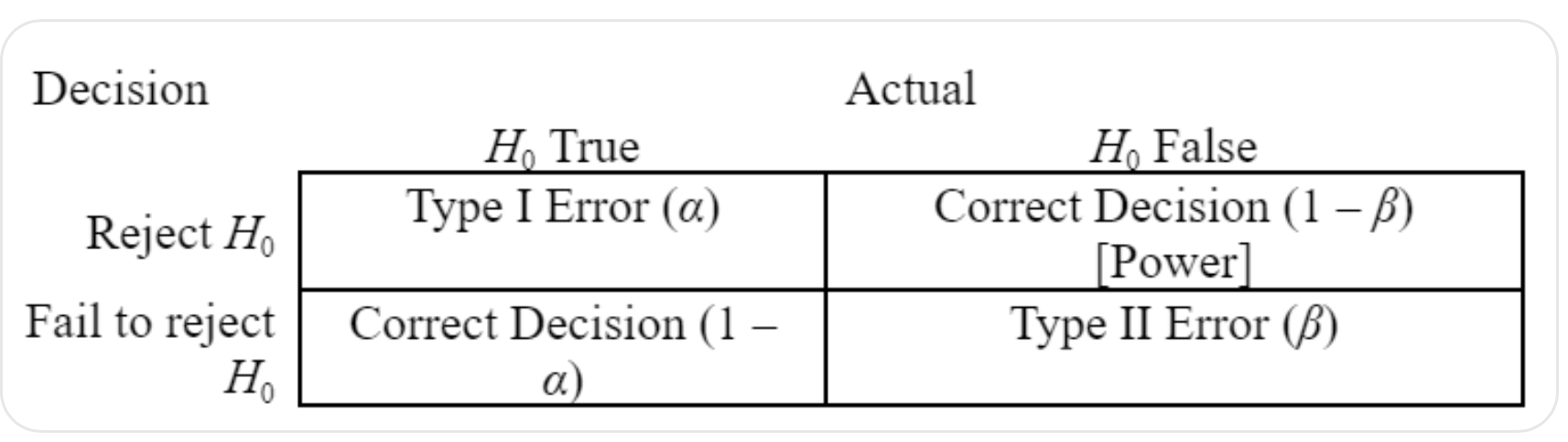
In statistical testing, there is a research hypothesis (what we want to test) and a null hypothesis (which assumes there is no difference). For example, a researcher might hypothesize that a new medication reduces headaches, while the null hypothesis assumes the medication has no effect. After conducting the study, there are two possible decisions: reject the null hypothesis or fail to reject it. If the results suggest the medication reduces headaches, we reject the null; if there is not enough evidence, we fail to reject it.

Whenever we make this decision, there is the possibility of error. A Type I error occurs when we reject the null hypothesis when it is actually true—for example, concluding that the medication works when it actually does not. The conditional probability of making a Type I error is designated as an alpha value, typically set as .05. This means the probability of making a Type I error is 5%. We can aim to reduce our alpha value to .01, however, this increases our risk of making a Type II error. A Type II error occurs when we fail to reject the null hypothesis, when the null hypothesis is false and the alternative hypothesis is true—for example, concluding the medication does not work when it actually does. This error is represented by beta (β). Statistical power is the probability of correctly rejecting a false null hypothesis and is equal to 1 – β.

The balance between Type I and Type II errors is important because depending on the study, it may be necessary to reduce alpha, thereby decreasing the chance of a Type I error but increasing the chance of a Type II error. For example, in a study exploring a medication with potentially serious side effects, reducing alpha to 0.01 might help researchers avoid falsely claiming the medication is effective when it is not (Type I error), even though this increases the risk of missing a truly effective treatment (Type II error).

Statistical Interaction / Simple effects, main effects, Interaction

In factorial designs (such as ANOVA), researchers examine the effects of two or more independent variables (factors) on a dependent variable. A statistical interaction occurs when the effect of one independent variable (IV) on a dependent variable (DV) depends on the level of another variable, known as a moderator. When a significant interaction effect is detected, it suggests that the simple effect of the IV on the DV varies as a function of the moderator. For example, imagine a study that measures exam scores, which is the dependent variable. The first independent variable may be the method of studying (flashcards vs. rereading notes), and the second independent variable may be time of day (morning vs. night). An interaction would mean the benefit of study method changes depending on the time of day. Suppose practice tests improve scores more than flashcards in the morning, but in the evening, both methods lead to similar scores. This interaction can be observed on a graph of plotted results, if the lines of the different levels of an IV do not run parallel.

Simple effects are follow-up tests performed when a significant interaction is found. A simple effect looks at the effect of one factor for those observations at only one level of the other factor. For instance, we might examine whether study method (flashcards vs. practice tests) has an effect within morning participants only, and then test the same comparison within evening participants. By breaking down the interaction into simple effects, researchers can “tease apart” how the two variables combine to influence the dependent variable.

Main effects refer to the effect of one factor on the dependent variable while ignoring the other factors. For example, The main effect of study method would look at whether flashcards or practice tests lead to higher scores overall, ignoring time of day. Similarly, the main effect of time of day would look at whether students perform better in the morning or evening, ignoring study method. Interactions are often more informative than main effects, because they show how variables combine to influence outcomes rather than just acting independently.

Z-scores

Z-scores are a form of linear transformation that changes raw scores into standardized scores and maintains the distribution of scores. They are calculated by subtracting the mean from a raw score and dividing by the standard deviation: z = (X - M) / SD. The distribution of z-scores has a mean of 0 and a standard deviation of 1. A z-score of 0 represents a score exactly at the mean, while positive or negative scores show how many standard deviations above or below the mean a score falls. For example, a z-score of 1 is one standard deviation above the mean, and -1 is one standard deviation below.

Z-scores are valuable because they allow us to compare scores that use different scales or measures, making test scores from different exams or studies directly comparable. Converting raw scores to z-scores standardizes the data, allowing comparisons across samples and between individuals. Z-scores also help identify outliers; because 95% of scores in a normal distribution fall between -2 and +2 standard deviations, any score beyond this range is considered unusual or extreme. In addition, z-scores can be used to find the percentile of a score, showing the percentage of scores that fall below it. They are also useful in computing statistics like correlation coefficients; for example, converting both GPA and study hours to z-scores allows a direct comparison despite the variables using different units.

Slope and intercept in bivariate regression

Regression is a statistical technique used to investigate how variation in one or more variables predicts or explains variation in another variable. A bivariate regression is if only one variable is used to predict or explain the variation in another variable. The formula of a bivariate regression is Ŷ = bX + a, where Ŷ is the predicted value of Y (the dependent variable), b is the slope of the regression, X is the value of the predictor variable (independent variable), and a is the intercept.

The slope of the regression (b) represents the amount of change in Ŷ associated with a one-unit change in X (the independent variable). The slope can be positive or negative and represents the steepness or rate of change in the line. For example, a slope of 3 is steeper than a slope of 1, indicating that more change happens in Ŷ as X changes. The intercept (a) is the value of Ŷ when X = 0. We can plug in any X value to get the predicted Y value (Ŷ). Importantly, the reason this equation uses Ŷ instead of Y is because the hat represents that there is error in our prediction. We can examine residuals (i.e., the difference between Ŷ and observed Y) by looking at this line and the actual Y values.

For example, let’s say an intercept of 15 and slope of 2.5 in a bivariate regression analysis investigating the effect of depression on anxiety was found. This would indicate that an anxiety score of 15 is found when depression scores are 0 and for each 1-unit increase of depression score predicts a 2.5 unit increase in anxiety score. 

Measures of central tendency (Mean, median, and mode)

Mean, median, and mode are different measures of central tendency and reflect where on the scale the distribution is centered. The mode can be defined simply as the most common score, that is, the score obtained from the largest number of subjects. Thus, the mode is that value of X that corresponds to the highest point on the distribution. It has advantages such as it is a score that actually occurred, it represents the largest number of people, and is unaffected by extreme scores. The median is the score that corresponds to the point at or below which 50% of the scores fall when the data are arranged in numerical order. By this definition, the median is also called the 50th percentile. The median location can be calculated by the equation: (N + 1) / 2. The median is also unaffected by extreme scores and is useful in studies where extreme scores occasionally occur but have no particular significance. The most common measure of central tendency is the mean, or average scores. It is the sum of the scores divided by the number of scores. The mean his highly affected by extreme scores, however, its advantages, such as being algebraically manipulable and providing more stable estimates of central tendency across samples compared to the median or mode, give evidence as to why it is so widely used.

For example, let’s say the data set includes 2, 2, 4, 5, and 7. The mode would be 2 because it occurs the most frequently. The median would be 4 because it is in the center of the distribution. The mean would be 4 because the sum of the numbers (20) divided by how many numbers occur (5) is 4

Homoscedasticity in regression vs Heteroscedasticity

Homoscedasticity (or the homogeneity of variance) is one of the assumptions in regression and refers to constant variance of residuals; there is a constant spread of residuals throughout all values of the independent variable (X). Ideally we want the variance for Y for each value of X to be constant. Homoscedasticity is examined using the plot of regression standardized predicted values by the regression standardized residuals (zpred x zresidual). In examining this plot, we want the scatter to be randomly distributed around 0 on the y-axis (regression standardized residuals). This is opposed to heteroscedasticity which is the difference in variance of residuals across values of X, and are not constant. We expect errors in prediction, but want errors to be random in nature and therefore uniformly distributed around the regression line. If there is a pattern in the distribution or tighter/larger discrepancies along different parts of the regression line then we likely have heteroscedasticity, which violates the assumption of homoscedasticity. 

Family-wise error rate / Post-Hoc

When making comparisons between group means, a “family” of conclusions is made. This might commonly be encountered when conducting post-hoc tests on an analysis, like an ANOVA, to better understand how specific groups might differ on an outcome. The family-wise error rate is the probability that these comparisons will result in at least one Type I error - which is rejecting the null hypothesis when the null is true. This is calculated by 1 – (1 – alpha) to the power of c, where c = comparisons. For example if alpha = .05 with 4 comparisons: 1— (1- .05) 4 = .185 meaning we have a 18.5% chance of making at least one type I error. Error inflation is created by multiple post-hoc comparisons made in a single experiment; as you conduct more contrasts, the family-wise error rate goes up. This is why researchers emphasize making post-hoc test decisions based in theory and practice and not searching for every possible comparison because multiple comparisons increase the family-wise error rate. A common way to control the family-wise error rate is the Bonferroni correction to utilize a more conservative alpha level based on the number of comparisons being made. The Bonferroni multiple-comparison procedure allows us to control the family-wise error rate by dividing our alpha level by the number of comparisons. While Bonferroni is the most stringent corrected, other post-hoc methods like Sidak (which allows for greater power than Bonferroni) and Tukey HSD can be used to decrease the likelihood of committing Type I errors.

Confidence intervals / 95% confidence interval around the mean  !!!!

A confidence interval gives an estimated range of values, which is likely to include an unknown population parameter. With a 95% confidence interval, we expect that 95% of our interval estimates, constructed from repeated random samples of the same size, will include the population parameter. Importantly, confidence intervals are statements of probability that the interval encompasses the target population parameter. Confidence intervals do not mean that the target statistic is within the interval. In other words, confidence intervals indicate the confidence we have in the process used to generate the interval, not the probability of the parameter lying within any particular interval. For example, imagine a study estimating the average exam score for all psychology majors at a university. A 95% confidence interval might be calculated as 75 to 85 points. This means the researchers are 95% confident that the true average score of all psychology majors falls within that range. It does not mean there is a 95% chance the true average lies within that range for this specific sample, but rather, if the study were repeated many times, 95% of the resulting intervals would contain the true average. Another example is with psychological testing. For example, when calculating an individual's score on the WISC, you provide confidence intervals to explain how certain we are that the score falls within that variable, which provides a more accurate description of where the true score likely falls, accounting for measurement error and sampling variability.

Multicollinearity in multiple regression !!!

Multicollinearity refers to predictor variables being correlated among themselves. For example, including both weight and BMI in the same regression model creates multicollinearity because BMI is derived from weight, so they are highly correlated and provide overlapping information. Multicollinearity increases the standard error of a regression coefficient, which increases the width of the confidence interval and decreases the t value for that coefficient. This is what is measured by the variance inflation factor (VIF). When two predictors are highly correlated, one has little to add over and above the other and only serves to increase the instability of the regression equation. Tolerance is the reciprocal of the VIF. So, we want a low value of VIF and a high value of Tolerance. Tolerance tells us the degree of overlap among the predictors, helping us to see which predictors have information in common and which are relatively independent. (The higher the tolerance, the lower the overlap.) Just because two variables substantially overlap in their information is not reason enough to eliminate one of them, but it does alert us to the possibility that their joint contribution might be less than we would like. Tolerance also alerts us to the potential problems of instability in our model. With very low levels of tolerance, the stability of the model and sometimes even the accuracy of the arithmetic can be in danger. In the extreme case where one predictor can be perfectly predicted from the others we will have what is called a singular covariance (or correlation) matrix . The most likely explanation for this is that one predictor has a tolerance of 0.00 and is perfectly correlated with others. In this case you will have to drop at least one predictor to break up that relationship. Such a relationship most frequently occurs when one predictor is the simple sum or average of the others, or where all p predictors sum to a constant.

Measures of Dispersion/Variability !!

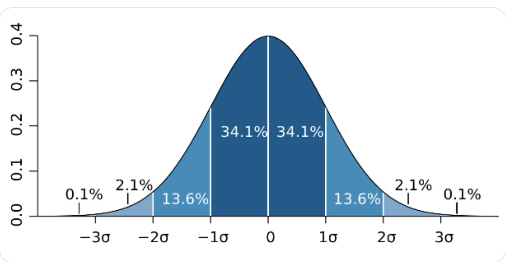
Measures of dispersion look at the variability around the median, the mode, the mean, or any other point. Some measures of dispersion are range, interquartile range, standard deviation, and variance. Range is the distance between the highest and lowest scores. It is heavily dependent on extreme scores, which may give a distorted picture of the variability in scores. Interquartile range (IQR) is obtained by discarding the upper 25% and the lower 25% of the distribution and taking the range of what remains. The point that cuts off the lowest 25% of the distribution is called the first quartile and point that cuts off the upper 25% of the distribution is called the third quartile. The difference between the first and third quartiles is the interquartile range. However, the interquartile range discards too much of the data. Variance refers to summing the squared deviations from the mean and divide by the number of scores (N-1 for sample, N for population). Variance allows us to observe how spread out our data points are from the mean, or the average squared deviation from the mean. Standard Deviation is defined as the positive square root of the variance for a sample and tells us, on average, how far each score deviates from the mean. The standard deviation has the advantage of reflecting variability in terms of the size of raw deviation scores, whereas the variance reflects variability in terms of squared deviation scores.  In a normal distribution, about 68% of values fall within one standard deviation of the mean, about 95% of the values fall within two standard deviations from the mean, and about 99.7% fall within three standard deviations from the mean.

ANOVA vs Regression !!!!

The Analysis of Variance (ANOVA) test is utilized to explore differences between or among sample means of two or more groups as well as examine the individual and interacting effects between multiple independent variables simultaneously. To use an ANOVA, it is important that the independent variable consists of two or more categorical, independent groups (e.g., treatment group). The dependent variable should be a continuous variable (i.e., depression). It not only asks about the individual effects of each variable separately, but also about the interacting effects of two or more variables. A statistical interaction occurs when the effect of one independent variable (IV) on a dependent variable (DV) depends on the level of another variable, known as a moderator. When a significant interaction effect is detected, it suggests that the simple effect of the IV on the DV varies as a function of the moderator. For example, imagine a study that measures exam scores, which is the dependent variable. The first independent variable may be the method of studying (flashcards vs. rereading notes), and the second independent variable may be time of day (morning vs. night). An interaction would mean the benefit of study method changes depending on the time of day. Suppose practice tests improve scores more than flashcards in the morning, but in the evening, both methods lead to similar scores. There are multiple assumptions that must be met in ANOVA. First, homoscedasticity, which indicates that both populations have the same variances. A second assumption is that the dependent variable for each group is normally distributed around the mean. The third assumption is that the observations are independent of one another.

Regression is a statistical method used to examine the relationship between one or more predictor variables (Indepndent variables) and a dependent variable. It is often used to determine how well predictor variables explain variation in the outcome variable and to predict values of the outcome based on known values of the predictors. The dependent variable is typically continuous, while the independent variables may be continuous or categorical. A bivariate regression uses one predictor, with the equation Y hat =bX + a, where Ŷ is the predicted value of Y (the dependent variable), the slope (rate and direction of change in Y per unit of X) and a is the intercept. The regression line, or line of best fit, summarizes the predicted values of Y for given X values and is often visualized using a scatterplot, allowing researchers to observe the strength, direction, and shape (linear vs. nonlinear) of the relationship. A key concept in regression is the residual, the difference between the actual value and the predicted value on the regression line. Residuals represent error in prediction, and examining them helps check assumptions in regression such as homoscedasticity, which requires constant variance of residuals across predictor levels. Overall, ANOVA answers the question of group differences, while regression answers the relationship between variables and how well one variable predicts another

ANOVA: define it —> talk about interaction, maybe simple effects and main effects.

Regression: define it —> talk about bivariate regression —> regression line, residuals, homoscedasiticty.

Residuals

Residuals are the differences between the actual observed values of the dependent variable (DV) and the values predicted by a regression model. In regression, we use one or more independent variables (IVs) to make predictions about the DV — and residuals tell us how far off each prediction was. Each residual is a numeric value that represents the error in prediction for a single data point. (residuals = observed DV - Predicted DV). Residuals are important because they show how much unexplained variability is left in the DV after accounting for what the model explains. The lower the residual the more accurate the predictions in your regression, which indicates your IVs are related to or predictive of the DV. Scatterplots with a line of best fit can help visualize residuals in a data set. An assumption in regression is homoscedasticity, which assumes that the variance of the residuals is consistent across the predictor. 

Box Plot

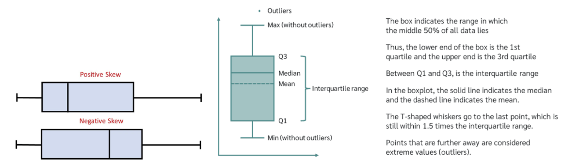
A box plot, also known as a box and whisker plot, was developed by John Tukey to examine the dispersion of data, specifically examining outliers around the median. A boxplot uses the 1^st and 3^rd quartiles which bracket the middle 50% of scores. The range between the 1^st and 3^rd quartiles is known as the interquartile range. We would draw a box around the 1^st and 3^rd quartiles, with a vertical line representing the median. Then, we would draw the whiskers of the box plot. The whiskers show the lower and upper quartiles of 25% of the data. The maximum and minimum are determined by the equation: 1.5xIQR of the 1^st and 3^rdquartiles. Any point beyond these is considered an outlier. Examining the box plot allows us to tell if the distribution is symmetric by examining whether the median lies in the center of the box. Skewness can also be determined by the length of the whiskers compared to one another. Outliers are determined as values outside the whiskers.

Outliers and their effects

Outliers are scores that significantly deviate from the rest of the data. These can be extreme values. Outliers sometimes represent errors in recording or scoring data, or actual issues with the participant. An example of an error causing an outlier is coding 98 for age instead of 28. Outliers affect the skewness of a distribution by pulling the distribution in the direction of the outliers. This means that the mean value is pulled toward the outliers. Outliers can be detected using visual techniques, like frequency distributions, scatterplots, and box plots, and statistical techniques like Cook’s D. To deal with outliers, we can correct the data entry or collection errors by double-entering the data. Researchers can also exclude extreme cases using trimmed means or winsorizing data. Further, outliers can be dealt with by removing the value completely.

Assumptions of ANOVA

The Analysis of Variance (ANOVA) test is utilized to explore differences between or among means of two or more groups as well as examine the individual and interacting effects between multiple independent variables. To use an ANOVA, it is important that the independent variable consists of two or more categorical, independent groups (e.g., ethnicity). The dependent variable should be a continuous variable (i.e., interval or ratio). After ensuring ANOVA is the right test for the independent/dependent variables, there are multiple assumptions that must be met. The first assumption is homogeneity of variance, or homoscedasticity, which indicates that both populations have the same variances. A second assumption is that the dependent variable for each group is normally distributed around the mean. The third assumption is that the observations are independent of one another. For repeated measures ANOVA, sphericity is another assumption that refers to examining the covariance matrix in which all covariances are equal; however, this assumption is rarely met.