Chapter 9: Aggregate Supply and Aggregate Demand

Comparative Statics for Microeconomics

• Price and quantity changes are the result, NOT the cause, of economic event

1. Start with one equilibrium situation (intersection of supply and demand, other things the same)

2. Change one variable

3. Compare resulting equilibrium situation (intersection of supply and demand after the change) in terms of price and quantity

Comparative Statics for Macroeconomics

• Changes in real GDP, unemployment, and inflation are the result, NOT the cause of economic events

1. Start with one equilibrium situation (intersection of aggregate supply and aggregate demand, other things the same)

2. Change one variable

3. Compare resulting equilibrium situation (intersection of aggregate supply and aggregate demand after the change) in terms of real GDP, unemployment, and inflation

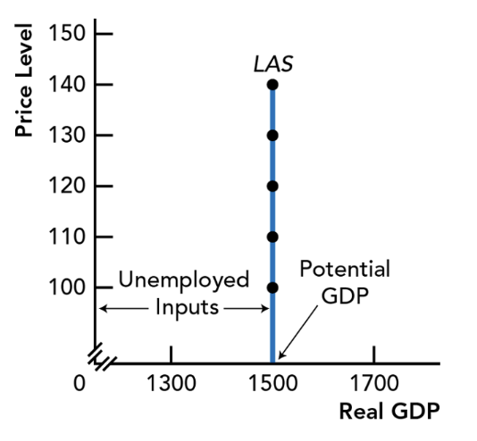
Long-Run Aggregate Supply (LAS)

Models the macroeconomic target outcomes of potential GDP and full employment with existing inputs

• Quantity of real GDP supplied when all inputs fully employed

• Long-run aggregate supply curve: vertical line at potential GDP — potential GDP does not change when price level changes

• Points on production possibilities frontier (PPF)

Time Periods for Macroeconomic Analysis

1. Long-Run: a period of time long enough for all prices and wages to adjust to equilibrium

• Economy at potential GDP

• The full employment outcome of coordinated smart choices

• Prices flexible in both input and output markets

2. Short-Run: a period of time when some input prices do not change

• All prices have not adjusted to clear all markets

• Prices fixed in input markets, but flexible in output markets

Macroeconomic players (consumers, businesses, government) make two kinds of plans for supplying realm GDP

1. Supply plans for existing input (With this new factory, how many workers does a business hire?)

2. Supply plans to increase input (Should the business build a new factory?)

Short-Run Aggregate Supply (SAS)

Quantity of real GDP macroeconomic players plan to supply at different price levels

Law of Short-Run Aggregate Supply: as price level rises, aggregate supply of real GDP increases

• Changes in price level cause movement along an unchanged short-run aggregate supply curve

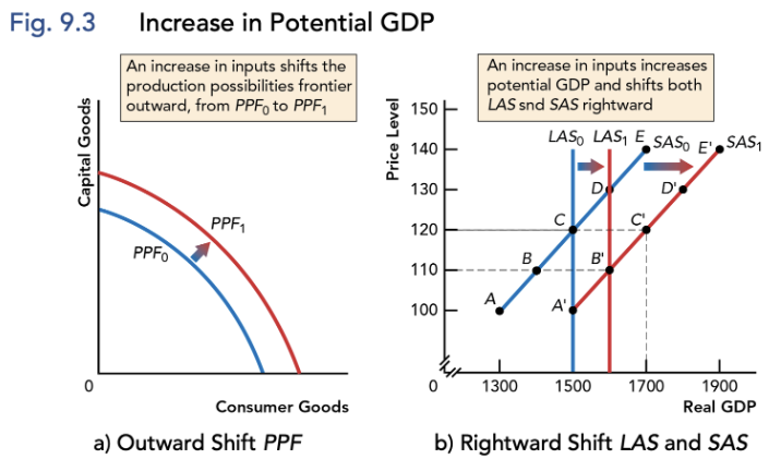
Movement of LAS and SAS

• Supply plans to increase quantity or quality of input cause increase in aggregate supply

• Changes in the quantity or quality of inputs shift both long-run aggregate supply curve (LAS) and short-run aggregate supply curve (SAS) in the same direction

• Both aggregate supply curves shift rightward for increase in inputs; shift leftward for decrease in inputs

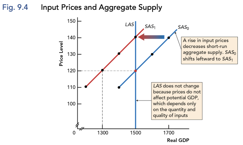
Changes in input prices…

Shift short-run aggregate supply curve (SAS) but do NOT shift long-run aggregate supply curve (LAS)

• Rising input prices shift SAS leftwards — decrease willingness to supply

• Falling input prices shift SAS rightwards — increase willingness to supply

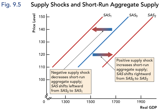
Supply Shocks

• Aggregate supply increases/decreases based on shocks (aggregate quantity supplied rises/falls based on price level)

Negative Supply Shocks: directly increase costs or reduce inputs, decreasing short-run aggregate supply — SAS shifts leftward

Positive Supply Shocks: directly decreases costs or improve productivity, increasing short-run aggregate supply — SAS shifts rightward

Aggregate Demand (AD)

Quantity of real GDP macroeconomic players plan to demand at different price levels

• There will be changes in aggregate demand if taxes changes

Law of Aggregate Demand: as price level rises, aggregate quantity of real GDP decreases

Fallacy of Composition

Makes macroeconomic law of aggregate demand different from microeconomic law of demand

• When prices rise for all Canadian products and services, only substitutes are important from R.O.W.

• Canadians buy more imports, and R.O.W buys fewer Canadian Exports

Planned Spending on Aggregate Demand = Planned C + Planned I + Planned G + Planned (X-IM)

Consumers plan to spend (C) a fraction of disposable income and save the rest

• Consumer spending is the largest, most stable component of aggregate demand

• Disposable income = income - taxes + transfers

Business plan investment spending (I) for new factories and equipment

• Investment spending plans quickly change (volatile) because easily postponed

• Can directly change aggregate demand and long-run aggregate supply

Government spending plan (G) for products and service set by budget

• Transfer payments are not part of G

• G as a percentage of real GDP stable since early 1990s

R.O.W spending plans (X) for Canadian exports

• Must subtract imports (IM) from all other planned spending to get net exports (X-IM)

Demand Shocks

Changes in factors, other than price level, that change aggregate demand and shift aggregate demand curve (AD)

• Expectations

• Interest Rates

• Government Policy

• GDP in R.O.W.

• Exchange Rates

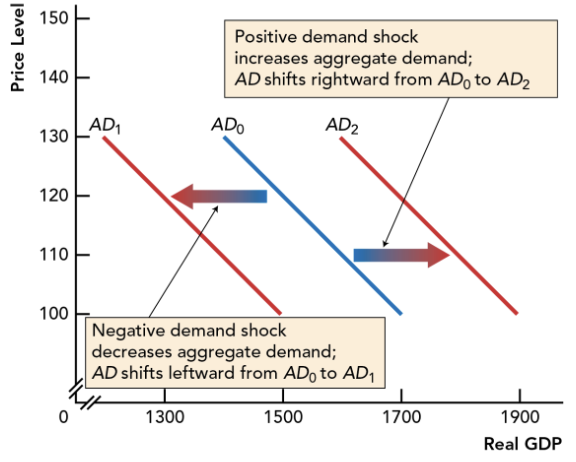
Negative Demand Shocks

Decrease aggregate demand — AD shifts leftward

• More pessimistic expectations (affect I)

• Higher interest rates (affect I or C)

• Lower government spending or higher taxes (affect G)

• Decreased in R.O.W. (affects X, IM)

• Higher value of Canadian dollar (affects X, IM)

Positive Demand Shocks

Increase aggregate demand — AD shifts rightward

• Les pessimistic expectations (affect I)

• Lower interest rates (affect I or C)

• Higher government spending or higher taxes (affect G)

• Increased in R.O.W. (affects X, IM)

• Lower value of Canadian dollar (affects X, IM)

SAS vs. AD vs. LAS

SAS: short-run supply plans by all macro players with fixed inputs

AD: short-rum demand plans by all macro players

LAS: a performance target, where all economists want to end up

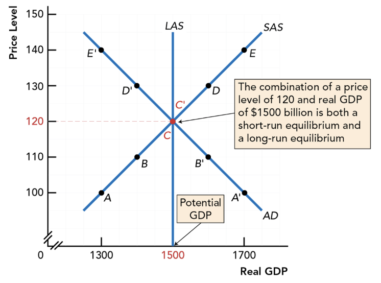
Short-Run and Long-Run Macroeconomic Equilibrium

In macroeconomic equilibrium, aggregate demand matches aggregate supply and there is no tendency to change

Short-Run Macroeconomic Equilibrium: with existing inputs is point wheres short-run aggregate supply (SAS) and aggregate demand (AD intersect

Long-Run Macroeconomic Equilibrium: with existing inputs is the point where SAS, AD, and LAS all intersect

• Aggregate quantity supplied and aggregate quantity demand of real GDP also equal potential GDP

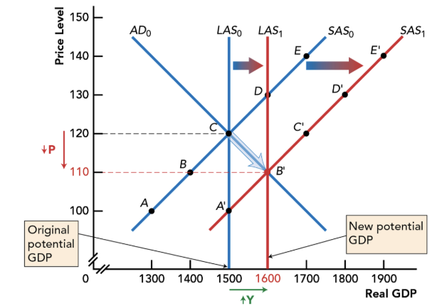
Economic Growth, Rising Living Standards, and Stable Prices

• For macroeconomic equilibrium over time with increasing inputs, business investment spending is key to steady growth in living standards, continued full employment, stable prices

  • Business investment that increases quantity and quality of inputs shifts both SAS and LAS rightward, potential GDP increases

  • Increased employment in new and improved factories increases incomes in input markets, so aggregate demand (AD) shifts rightward

  • New LAS, SAS, and AD curves all intersect, so full employment continues with stable prices, growth in living standards from increased potential GDP

Four mismatches between aggregate demand and aggregate supply move the economy away from long-run equilibrium targets

1. Negative demand shocks

2. Positive demand shocks

3. Negative supply shocks

4. Positive supply shocks

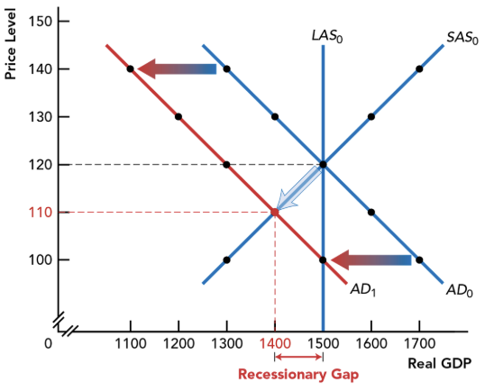
1. Negative Demand Shocks

• Cause a recessionary gap

• Falling average prices

• Decreased real GDP (Y)

• Increased unemployment

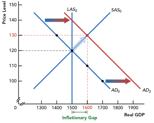
2. Positive Demand Shocks

• Cause inflationary gap

• Rising average prices

• Increased GDP (Y)

• Decreased unemployment

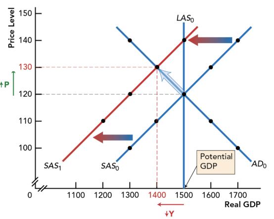
3. Negative Supply Shocks

• Cause stagflation

• Rising average prices

• Decreased GDP (Y)

• Increased unemployment

Positive Supply Shocks

• Falling average prices

• Increased GDP (Y) 

• Continued full employment

Using AS/AD Model to Think Like an Economist

1. To analyze any economic situation, always start in long-run macroeconomic equilibrium, where LAS, SAS, and AD all intersect, and do comparative statics

2. Remember LAS is different from SAS and AD; LAS is a performance target, SAS and AD are plans

3. Model a macroeconomic event as one of the four possible shocks — positive/negative aggregate supply/demand shocks

4. At new short-run equilibrium, examine the results of the shock on real GDP, unemployment, inflation