MM - Chapter 7: Lossy Compression: Transform coding

wat is lossy compression

• The compressed data is not the same as the original data, but a close approximation of it

• Yields a much higher compression ratio than that of lossless compression

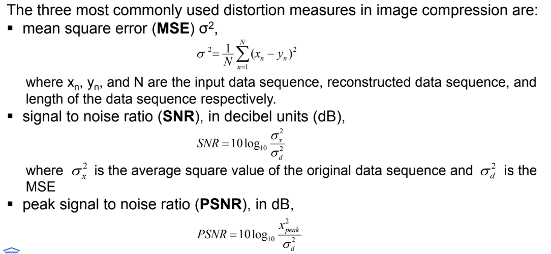
Measuring and comparing image quality (3 gebruikte maten)

(nogmaals) wat is quantization in de context van lossy compression?

Wat zijn de drie main forms van quatization?

Reduce the number of distinct output values to a much smaller set

• e.g., from Analogue to Digital (cf. Chapter 5)

• here: quantize already digitized samples to reduce dynamic range

Main source of the “loss” in lossy compression

Three main forms of quantization

• uniform: midrise and midtread quantizers

• non-uniform: companded quantizer, Lloyd-Max

• Vector Quantization

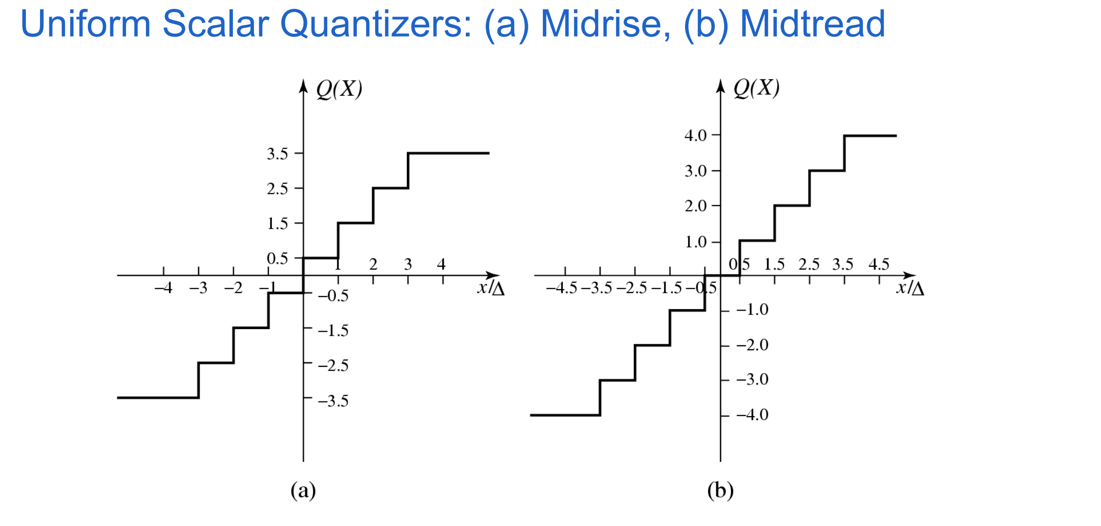
uniform scalar quantization

A uniform scalar quantizer partitions the domain of input values into equally spaced intervals, except possibly at the two outer intervals.

• length of each interval is referred to as the step size, denoted by the symbol Δ

• the output or reconstruction value corresponding to each interval is typically taken to be the midpoint of the interval

Two types of uniform scalar quantizers:

• midrise quantizers have even number of output levels.

• midtread quantizers have odd number of output levels, including zero as one of them

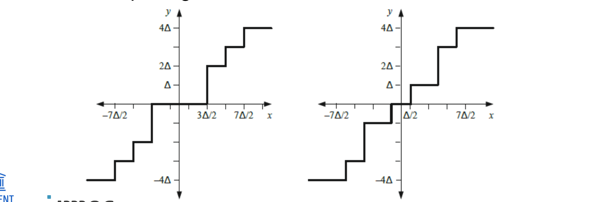
non-uniform scalar quantization

Non-uniform step sizes can be beneficial when:

• signal does not exhibit a uniform PDF

• signal ranges are known to contain excess noise

• there is a need to incorporate non-linear amplitude mapping

  • cf. A law (Chapter 5)

• there is a desire to map a range of low-level signals to zero

Two common non-uniform quantizers

• Deadzone (left) and Lloyd-Max (right)

• Lloyd-Max minimizes distortion by adopting the quantizer to the PDF of the input signal

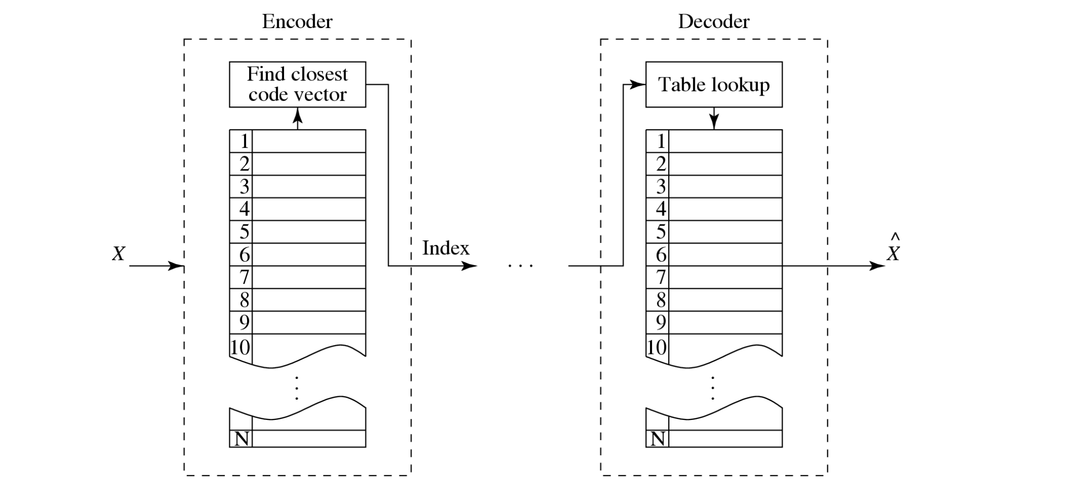
vector quantization

According to Shannon’s original work on information theory, any compression system performs better if it operates on vectors or groups of samples rather than individual symbols or samples

• Form vectors of input samples by simply concatenating a number of consecutive samples into a single vector

• VQ defines a set of code vectors with n components

  • instead of single reconstruction values as in scalar quantization

• A collection of these code vectors form the codebook

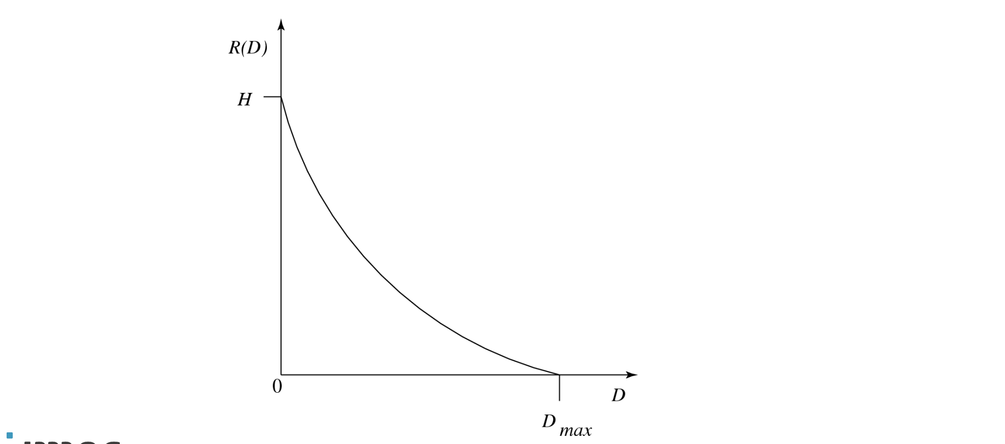
Rate-Distortion Theory

Framework to study of trade-offs between Rate and Distortion

• typical Rate Distortion Function:

  

Bit rate for any compressed sequence depends on

• encoding algorithm

  • differential or not, intra vs. inter, supported motion estimation, available block sizes, ...

• content

  • high spatio-temporal activity typically requires more bits

• selected encoding parameters

  • resolution, frame rate, quantizer, block size choice, combining inter and intra, ...

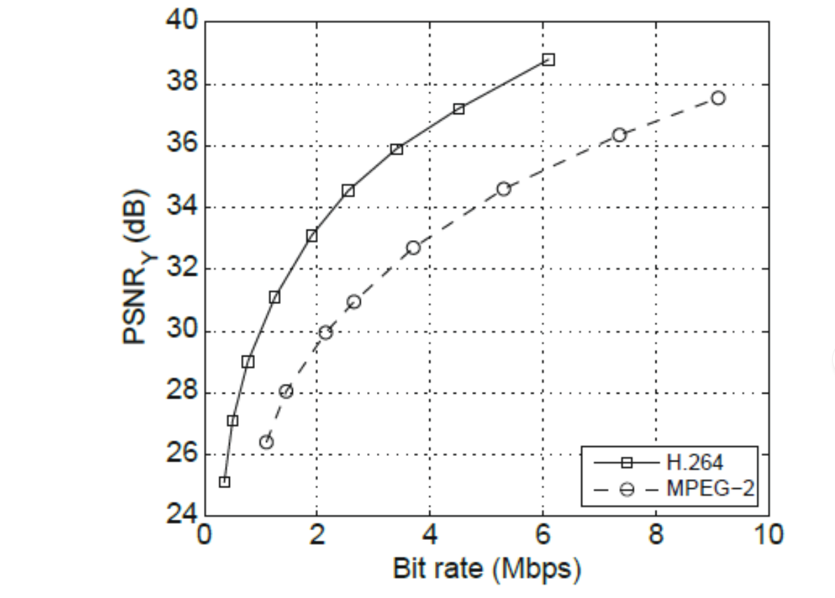
Often, Rate-Quality curves are used

principles of decorrelating transforms

The rationale behind transform coding:

• If C is the result of a linear transform A of the input vector X in such a way that the components of C are much less correlated, then C can be coded more efficiently than X

• If most information is accurately described by the first few components of a transformed vector, then the remaining components can be coarsely quantized, or even set to zero, with little signal distortion

  

What did just happen?

• rotating axes effectively decorrelates the data

  • x0 vs. x1 compared to c0 vs. c1

• small values can be set to zero

  • → sparse set of coefficients containing most of the information

• remaining values can be quantized

  • compression (!)

This is the essence of transform-based data compression

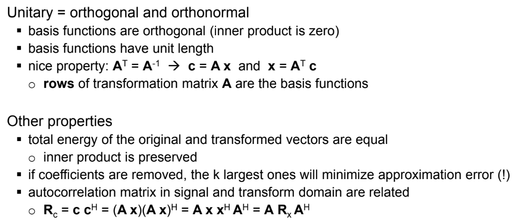
unitary transforms (??)

A signal x can be approximated using a linear combination of basis functions bk​ (cf. Fourier analysis)

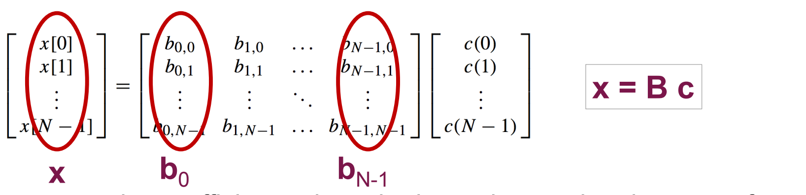
Typically, we want to compute the coefficients given the input data and a given set of basis funtions: c = A x, and hence: x = A^−1 c, which means that B = A^−1

A → transformation matrix
c → transform coefficients
columns of B (=A−1A−1) → basis functions of the transform

basic transforms: Walsh-Hadamard transform

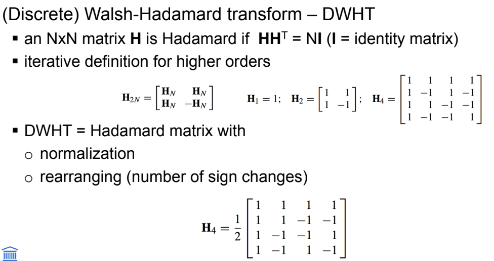
veel vb dias en cursus

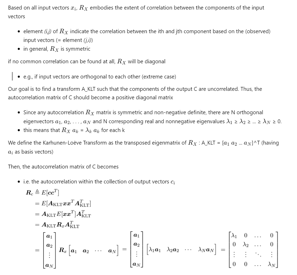
the Karhunen-Loève Transform (KLT) (????)

The Karhunen-Loève transform is a reversible linear transform that exploits the statistical properties of the vector representation

• it optimally decorrelates the input signal

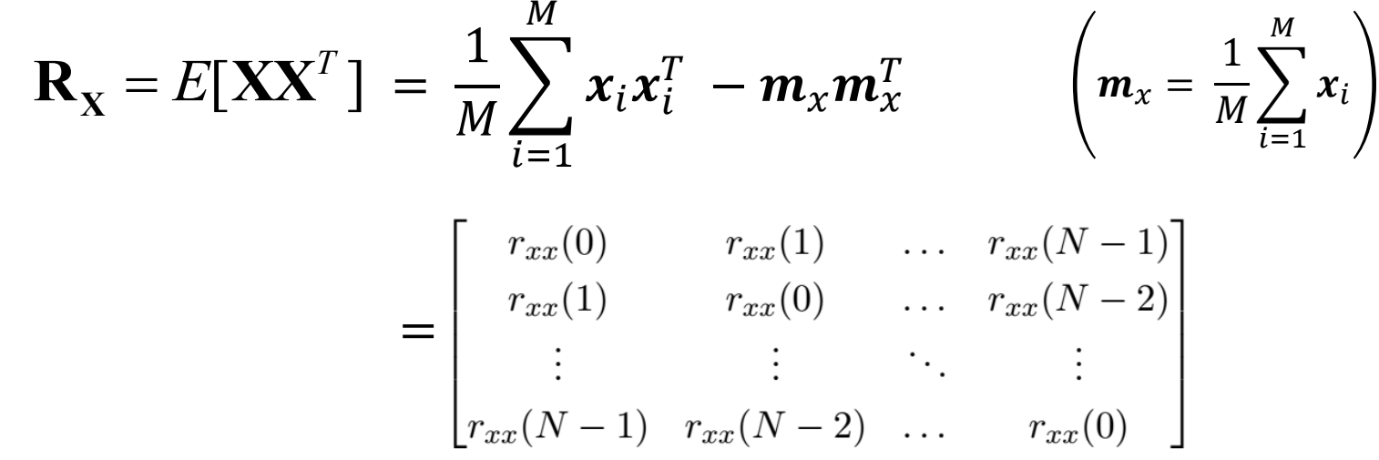
To understand the optimality of the KLT, consider the autocorrelation matrix Rx​ of the input vectors xi defined as

Discrete Cosine Transform

• Most widely used unitary transform for image/video coding

• Like Fourier, it provides frequency information about a signal, but

  • DCT is real-valued

  • DCT doesn’t introduce artifacts due to periodic extension of the signal

• DCT is not as useful as the DFT for frequency-domain analysis

• DCT performs exceptionally well for signal compression

• DCT has very good energy compaction properties, and approaches the KLT for correlated image data

  • without the need to signal the transform basis functions

The DCT of x[n] can be derived by applying the DFT on the symmetrically extended (mirrored) signal x1[n]

• this even extension cancels out the imaginary part of the DFT (sines)

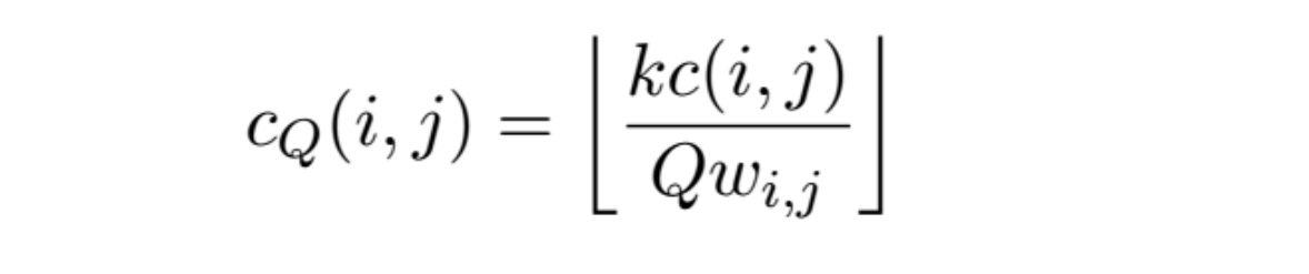
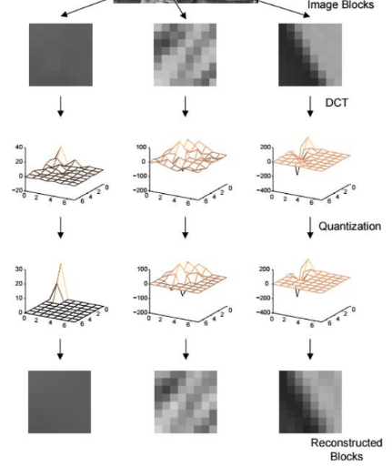
Quantization of DCT coefficients

DCT itself does not provide compression

• DCT concentrates energy of the signal in a few high-valued coefficients

  • retain important transform coefficients (no or little quantization)

  • coarser quantization for unimportant coefficients

    • or even remove small coefficients (set to zero)

• Use of coefficient-dependent weighting of the quantizer step-size

DCT implementation

Trade-off between decorrelation performance and complexity

• decorrelation performance depends on transform size, but also on autocorrelation surface characteristics (content, resolution, etc.)

• typically between 4x4 and 16x16

• JPEG uses 8x8

Efficient impelmentations exist to reduce the DCT complexity