Deep learning Interview Questions

What is deep learning?

Deep learning is a subset of machine learning, inspired by the structure of the human brain, used to train artificial neural networks from vast amounts of data.
Deep learning is a branch of machine learning that is made up of a neural network with three or more layers:

• Input layer: Data enters through the input layer.

• Hidden layers: Hidden layers process and transport data to other layers.

• Output layer: The final result or prediction is made in the output layer.

Example of deep learning: Self-driving cars, chatbot like Chatgpt, Facial recognition

What is AI?

AI is a method of building smart machines that are capable to think like human and mimic their actions.

What is machine learning?

Machine learning is an application of AI that allows machines to automatically learn and improve with experience.

How does Deep learning differ from traditional machine learning?

1. Feature Extraction:

   Traditional machine learning often linear models like logistic regression, decision trees, and support vector machines. These models rely on manual feature extraction, while deep learning: Utilizes complex architectures like neural networks with many layers (hence "deep"). These models automate this process, excelling with large datasets.
   

2. Data Requirements:

   • Traditional Machine Learning: Often effective with smaller datasets. These models can perform well when the data is limited but well curated.

   • Deep Learning: Requires large amounts of data to perform well, as the models need to learn potentially complex patterns from scratch.

What is neural network?

A neural network is a computational model designed to simulate human learning, inspired by the brain’s biological neural networks.

Structure and function: Consists of interconnected layers of neurons, adjusts connections (weights) during training, and is instrumental in complex tasks like image and speech recognition.

1. Input layer: is responsible to accept the inputs in various formats

2. Hidden layer: is responsible for extracting features and hidden patterns from the data

3. Output layer: produces the desired output after completing the entire processing of data.

What is perceptron?

A perceptron is a binary classification algorithm proposed by Frank Rosenblatt. It consists of single layer of artificial neurons that take input values, apply weights and generate an output.

The perceptron is typically used for linearly separable data, where it learns to classify inputs into two categories based on a decision boundary. It finds applications in pattern recognition, image classification, and linear regression. However, the perceptron has limitations in handling complex data that is not linearly separable.

What is epoch and iteration?

One epoch is when an entire dataset is passed forward and backward through the neural network only once.

Another way to define an epoch is the number of passes a training dataset takes around an algorithm. One pass is counted when the data set has done both forward and backward passes. 

The number of epochs is considered a hyperparameter. It defines the number of times the entire data set has to be worked through the learning algorithm. 

Example of an Epoch

Let's explain Epoch with an example. Consider a dataset that has 200 samples. These samples take 1000 epochs or 1000 turns for the dataset to pass through the model. It has a batch size of 5. This means that the model weights are updated when each of the 40 batches containing five samples passes through. Hence the model will be updated 40 times.

Iteration

The total number of batches required to complete one Epoch is called an iteration. The number of batches equals the total number of iterations for one Epoch. 

Here is an example that can give a better understanding of what an iteration is. 

Say a machine learning model will take 5000 training examples to be trained. This large data set can be broken down into smaller bits called batches. 

Suppose the batch size is 500; hence, ten batches are created. It would take ten iterations to complete one Epoch. 

Batch

The batch is the dataset that has been divided into smaller parts to be fed into algorithm and is a hyperparameter.

Types of Neutral network

Long short-term memory (LSTM) networks

LSTM networks are a type of recurrent neural network (RNN) designed to capture long-term dependencies in sequential data. LSTM networks have memory cells and gates that allow them to retain or forget information over time selectively. This makes LSTMs effective in speech recognition, natural language processing, time series and translation. The challenge with LSTM networks lies in selecting the appropriate architecture and parameters and dealing with vanishing or exploding gradients during training. Radial Basis Function (RBF) Neural Network

The RBF neural network is a feedforward neural network that uses radial basis functions as activation functions. RBF networks consist of multiple layers, including an input layer, one or more hidden layers with radial basis activation functions and an output layer. RBF networks excel in pattern recognition, function approximation, and time series prediction. However, challenges in training RBF networks include selecting appropriate basis functions, determining the number of basis functions, and handling overfitting.

Artificial Neural Network (ANN)

Artificial Neural Network or ANN, is a group of multiple perceptrons/neurons at each layer. ANN is also known as a Feed-Forward Neural network because inputs are processed only in the forward direction. ANN consists of 3 layers - Input, Hidden, and output. ANN can be used to solve problems related to Tabular data, Image data, and text data.

Advantages of Artificial Neural Network (ANN)

Artificial Neural Network is capable of learning any nonlinear function. Hence, these networks are popularly known as Universal Function Approximators. ANNs have the capacity to learn weights that map any input to the output.

One of the main reasons behind universal approximation is the activation function. Activation functions introduce nonlinear properties to the network. This helps the network learn any complex relationship between input and output.

Challenges with Artificial Neural Network (ANN)

• While solving an image classification problem using ANN, the first step is to convert a 2-dimensional image into a 1-dimensional vector prior to training the model. This has two drawbacks:

  • The number of trainable parameters increases drastically with an increase in the size of the image.

  • In the above scenario, if the size of the image is 224*224, then the number of trainable parameters at the first hidden layer with just 4 neurons is 602,112. That’s huge!

  • ANN loses the spatial features of an image. Spatial features refer to the arrangement of the pixels in an image.

Recurrent Neural Network (RNN)

Let us first try to understand the difference between an RNN and an ANN from the architectural perspective:

A looping constraint on the hidden layer of ANN turns to RNN.

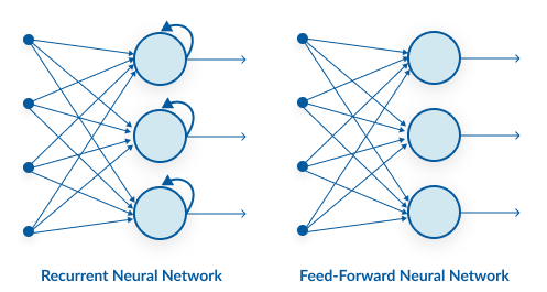As you can see here, RNN has a recurrent connection to the hidden state. This looping constraint ensures that sequential information is captured in the input data. We can use recurrent neural networks to solve the problems related to: time series data, text data, audio data.

Advantages of Recurrent Neural Network (RNN)

• RNN captures the sequential information present in the input data i.e. dependency between the words in the text while making predictions.

• RNNs share the parameters across different time steps. This is popularly known as Parameter Sharing. This results in fewer parameters to train and decreases the computational cost. As shown in the above figure, 3 weight matrices – U, W, V, are the weight matrices that are shared across all the time steps.

Challenges with Recurrent Neural Networks (RNN)

Deep RNNS (RNNs with a large number of time steps ) also suffer from the vanishing and exploding gradient problem which is a common problem in all the different types of neural networks.

Convolution Neural Network (CNN)

Convolutional neural networks (CNN) are all the rage in the deep learning community right now. These CNN models are being used across different applications and domains, and they’re especially prevalent in image and video processing projects.

The building blocks of CNNs are filters a.k.a kernels. Kernels are used to extract the relevant features from the input using the convolution operation.

Advantages of Convolution Neural Network (CNN)

• CNN learns the filters automatically without mentioning it explicitly. These filters help in extracting it explicitly. These filters help in extracting the right and relevant features from the input data.

• 

• CNN captures the spatial features from an image. Spatial features refer to the arrangement of pixels and the relationship between them in an image. They help us in identifying the object accurately, the location of an object, as well as its relation with other objects in an image.

• CNN also follows the concept of parameter sharing. A single filter is applied across different parts of an input to produce a feature map.

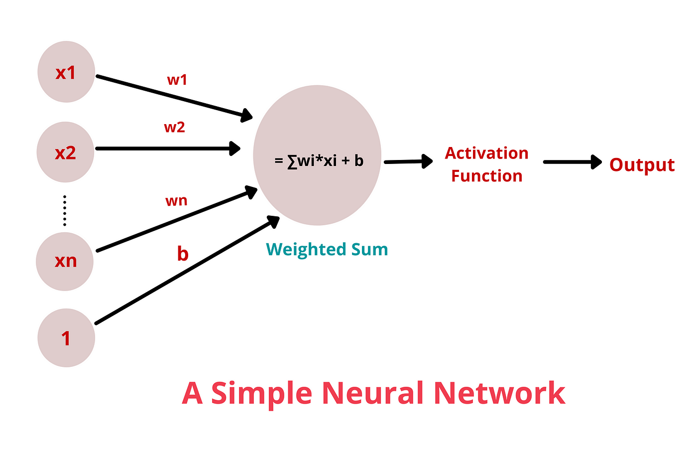
Explain the concept of a neuron in Deep Learning.

Neural networks consist of input, hidden and output layers, each layer transforming data into more abstract forms.

1. Inputs: Each neuron receives multiple inputs from the data or from the outputs of neurons in the previous layer. These inputs can represent raw data features or abstract features derived in earlier layers.

2. Weights: Each input is associated with a weight, which is a parameter that signifies the importance or strength of the input in the neuron's overall computation. The neuron's behavior is largely determined by these weights.

3. Bias: In addition to weighted inputs, a neuron has a bias term, which allows the neuron to shift the activation function to the left or right, which may be critical for successful learning.

4. Weighted Sum: The neuron computes a weighted sum of its inputs, which is the sum of each input multiplied by its corresponding weight. This sum is then adjusted by the bias. The formula for this computation is:

   where xi are the inputs, wi are the weights, b is the bias, and is the number of inputs to the neuron.5. Activation Function: The weighted sum is then passed through an activation function. The activation function is a non-linear transformation that determines the output of the neuron. Common activation functions include:

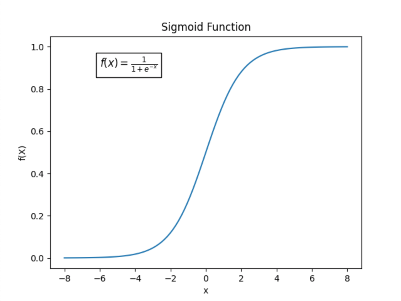
   1. Sigmoid: Maps the input to a range between 0 and 1, making it useful for binary classification.

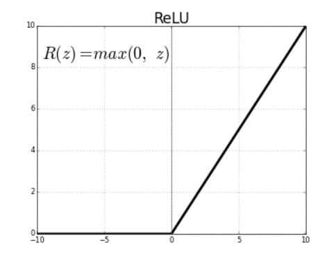
   2. ReLU (Rectified Linear Unit): Outputs the input directly if it is positive, otherwise, it outputs zero. It is the most commonly used activation function in deep learning due to its computational efficiency and effectiveness.

   3. Tanh (Hyperbolic Tangent): Maps the input to values between -1 and 1.

The choice of activation function affects how the network learns and performs.

Explain architecture of neural networks in simple way.

A neural network is a multi-layer structured model and each layer transforms the input data step by step think of an assembly line where every stage adds more complexity to the previous stage and the detail and the complexity add more value to the ability of the model to perform predictions.

1. The input layer is the first layer in a neural network. The input layer is the first layer in a neural network

2. Between the input layer and the output layer, there are one or more hidden layers. Each neuron in these layers receives inputs from the neurons of the previous layer, processes the inputs, and passes the output to the next layer. The hidden layers are where the network learns to represent complex patterns by adjusting the weights and biases through training.

3. Neurons in one layer connect to neurons in the next layer. These connections are associated with weights that adjust as the network learns during training. The strength of these connections (weights) determines how much influence one neuron has on another.

4. Each neuron applies an activation function to its input sum (the weighted sum of its inputs plus a bias term) to introduce non-linearities into the model. This is crucial because it allows the network to learn and model more complex patterns.

5. The output layer is the final layer in a neural network. which represents the prediction or decision made by the network based on the input data.

   

What is activation function in neural network?

An activation function in a neural network is a crucial component that introduces non-linearity into the network's operations. Without activation functions, a neural network would essentially be a linear regression model, which limits its ability to model complex patterns and interactions in data. Activation functions allow neural networks to learn and perform more complex tasks by enabling them to approximate non-linear functions. Most real-world data are non-linear, so this property is crucial for effective modeling.

Popular activation functions

• Sigmoid Function, Tanh function

• ReLU and Leaky ReLU

Name few popular activation functions and describe them.

Sigmoid function

• Characteristics: It outputs values between 0 and 1, which mimic probability values. It is historically used for binary classification in the output layer of a neural network. It is especially useful for models where we need to predict the probability as an output since the probability of anything exists only between the range of 0 and 1

Hyperbolic Tangent (Tanh) function:

• Characteristics: It outputs values between -1 and 1. It is similar to the sigmoid but provides better training performance for hidden layers because it centers the data, improving the efficiency of gradient descent.

• It is zero-centered, making it easier to model inputs that have strongly negative, neutral, and strongly positive values.

• 

Rectified Linear Unit (ReLu)

• It has become popular recently due to its relatively simple computation. This helps to speed up neural networks and seem to get empirically good performance, which makes it a good starting choice for the activation function.

• The Relu function is a max(0,x) function and is a piecewise function with all inputs less than 0 will be 0, which will not activate any of the negative neurons, and all inputs greater than or equal to 0 will be activated exactly the set scores.

• Applications: Widely used in most CNN (Convolutional Neural Network) and deep learning architectures due to its simplicity and efficiency.

Leaky ReLu

• Not only activates the positive scores but also activate the negative scores, which prevent the neurons from dying. It achieves this by having a small negative slope like 0.01 when the input is less than zero.

What happens if you do not use any activation functions in a neural network?

Absence of activation functions reduces a neural network to a simple linear regression model. The network becomes incapable of handling complex, non-linear data, limiting its real-world applicability.

Describe how training of basic neural networks works

1. Forward Pass:

The training process starts by feeding the input data is processed through neurons, using weighted sums and activation functions, to produce an output.

2. Loss calculation:

Once the network has produced its outputs, the next step is to calculate the loss or error. The loss function is chosen based on the specific task (e.g. mean squared error for regression, cross-entropy loss for classification). It measures how far the network’s predictions are from the actual target values.

3. Backpropagation:

To improve its predictions, the network needs to adjust its weights and biases. This adjustment is done using backpropagation, which is a method of applying the chain rule to find the gradient of the loss function with respect to each weight and bias in the network. The gradient tells us how the loss would change if the weights and biases were increased or decreased slightly and they guide the update process.

4. Weight Update

The weights are updated using the gradients calculated during backpropagation. This is typically done using an optimization algorithm like Gradient Descent or its variants (e.g., Stochastic Gradient Descent, Adam).Here, w is a weight, a is the learning rate (a small number that determines how much the weights are adjusted during each update), and (aerror/aws) is the gradient of the loss function with respect to w .

What is gradient descent?

Gradient descent is an optimization algorithm that we are using both machine learning and deep learning in order to minimize the loss function of our model, which means we are improving the model parameters in order to minimize the cost function and produce highly accurate predictions.

What is the function of an optimizer in deep learning?

In deep learning, optimizer is a crucial component in which network updates its weight based on the loss function, which measures how well the model is performing.

Different strategies:

• Gradient Descent: The simplest form, where weights are updated in the opposite direction of the gradient of the loss function.

• Stochastic Gradient Descent (SGD): An improvement over gradient descent, using a subset of data to estimate the gradient, which speeds up computation and can help avoid local minima.

• Momentum: Builds on SGD by incorporating the direction of previous gradients to speed up convergence and reduce oscillations.

• Adaptive Learning Rate Methods: Optimizers like AdaGrad, RMSprop, and Adam adjust the learning rate for each parameter, allowing for more fine-tuned updates based on their individual behaviors.

What is cost function

The cost function or loss function measures the accuracy of the network. The cost function tries to penalize the network when it makes errors.

What is backpropagation, and why is it important in Deep Learning?

Backpropagation is a method for training neural networks, allowing them to learn from errors by updating parameters (weights and biases).

Here's a more detailed explanation of backpropagation and its importance:

1. Forward pass: During the forward pass, input data is fed through the network, and the output is computed based on the current parameters.

2. Error calculation: The network's output is compared to the desired output (ground truth), and an error is calculated using a loss function, such as mean squared error or cross-entropy loss.

3. Backward pass: In the backward pass, the error is propagated backwards through the network. Using the chain rule of calculus, the gradients of the error with respect to each parameter are computed layer by layer, starting from the output layer and moving towards the input layer.

4. Parameter update: Once the gradients are computed, an optimization algorithm, such as gradient descent, is used to update the parameters in a direction that minimizes the error. The learning rate controls the step size of the parameter updates.

5. Iteration: Steps 1-4 are repeated for multiple iterations (epochs) over the training data until the network converges to a satisfactory level of performance.

The importance of backpropagation in deep learning:

1. Efficient gradient computation: Backpropagation allows for efficient computation of gradients in deep neural networks with many layers and parameters. Without backpropagation, computing these gradients would be computationally intractable.

2. Enables learning in deep networks: By providing a way to update the parameters based on the error, backpropagation enables deep neural networks to learn complex patterns and representations from data.

3. Scalability: Backpropagation scales well to large datasets and deep network architectures, making it suitable for training state of the art models in various domains, such as computer vision, natural language processing, and speech recognition.

4. Flexibility: Backpropagation can be applied to different network architectures, loss functions, and optimization algorithms, making it a versatile algorithm for training neural networks.

How is backpropagation different from gradient descent?

Backpropagation is process of computing the gradients to understand how much a change in the loss function is there when we are changing the model parameters

Gradient descent: Optimization algorithm that uses this gradient to adjust weights and minimize the loss.

The relationship between backpropagation and gradient descent:

• Backpropagation and gradient descent work together to train neural networks.

• Backpropagation computes the gradients, which are then used by gradient descent to update the network's parameters.

• The gradients provided by backpropagation guide gradient descent in finding the optimal parameter values that minimize the network's error.

Describe what vanishing gradient problem is and it’s impact on NN

The vanishing gradient problem is a challenge that arises when training deep neural networks using backpropagation and gradient-based optimization methods. Vanishing gradients happens when gradients of the network’s loss function weight parameters become very small, approaching to zero as they are propagated back through deep neural network during training., effectively preventing the network from learning or updating those parameters.

How does the vanishing gradient problem occur ?

The vanishing gradient problem is exacerbated by the depth of the network. As the number of layers increases, the gradients have to pass through more layers, leading to a greater chance of them vanishing before reaching the earliest layers.

Let's consider a deep neural network with L layers, and let's focus on the gradient of the loss function with respect to the weights in the first layer (W₁). Using the chain rule, the gradient can be expressed as:

∂Loss/∂W₁ = (∂Loss/∂Aₗ) (∂Aₗ/∂Aₗ₋₁) ... (∂A₂/∂A₁) (∂A₁/∂W₁)

where Aᵢ represents the activations of layer i.

If the derivatives of the activation functions (∂Aᵢ/∂Aᵢ₋₁) are small (< 1) for most layers, the gradient ∂Loss/∂W₁ will be a product of many small terms, resulting in a very small value. As the number of layers (L) increases, the gradient will vanish exponentially.

Method to overcome the vanishing gradient problem

The vanishing gradient problem is caused by the derivative of the activation function used to create the neural network. The simplest solution to the problem is to replace the activation function of the network. Instead of sigmoid, use an activation function such as ReLu.

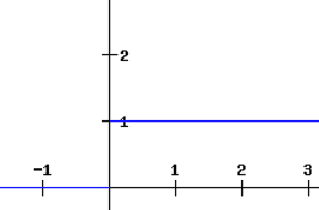
1. Rectified Linear Units (ReLU) are activation functions that generate a positive linear output when they are applied to positive input values. If the input is negative, the function will return zero.The derivative of a ReLU function is defined as 1 for inputs that are greater than zero and 0 for inputs that are negative. The graph shared below indicates the derivative of a ReLU function

Improved activation functions: Using activation functions like ReLU (Rectified Linear Unit) or its variants, which have gradients equal to 1 for positive inputs, helps alleviate the vanishing gradient problem by preventing gradient saturation. The problem with the use of ReLU is when the gradient has a value of 0. In such cases, the node is considered as a dead node since the old and new values of the weights remain the same. This situation can be avoided by the use of a leaky ReLU function which prevents the gradient from falling to the zero value.
2. Careful weight initialization: Initializing the network's weights using techniques like Xavier initialization or He initialization can help prevent the gradients from vanishing or exploding during the initial stages of training.

3. Batch normalization: Normalizing the activations of each layer can help maintain the gradients' magnitudes and reduce the impact of the vanishing gradient problem.

4. Skip connections: Architectures like ResNet (Residual Networks) and Highway Networks introduce skip connections that allow gradients to flow more easily from later layers to earlier layers, mitigating the vanishing gradient problem.

What is the connection between various activation functions and vanishing gradient problem?

Let's explore the connection between some common activation functions and the vanishing gradient problem:

1. Sigmoid activation function:

   -The sigmoid function, defined as f(x) = 1 / (1 + exp(-x)), has a gradient that is always between 0 and 0.25.

   -For input values that are very positive or very negative, the sigmoid function saturates, and its gradient becomes close to zero.

   -When the gradients are propagated through multiple layers with sigmoid activations, they get multiplied by these small values, leading to the vanishing gradient problem.

2. Hyperbolic tangent (tanh) activation function

   -The tanh function, defined as f(x) = (exp(x) - exp(-x)) / (exp(x) + exp(-x)), has a gradient that is always between 0 and 1.

   -Similar to the sigmoid function, the tanh function saturates for very positive or very negative input values, and its gradient becomes close to zero.

   -The vanishing gradient problem can also occur in networks with tanh activations, as the gradients get multiplied by small values during backpropagation.

3. Rectified Linear Unit (ReLU) activation function:

   -The ReLU function, defined as f(x) = max(0, x), has a gradient of 1 for positive input values and 0 for negative input values.

   -ReLU does not suffer from saturation for positive input values, which helps alleviate the vanishing gradient problem.

   -However, ReLU can suffer from the "dying ReLU" problem, where the gradients become zero for negative input values, potentially leading to some neurons becoming permanently inactive.

4. Leaky ReLU and Parametric ReLU activation functions:

   -Leaky ReLU and Parametric ReLU are variants of the ReLU function that introduce a small slope for negative input values, instead of a flat zero.

   -These activation functions help mitigate the dying ReLU problem by allowing gradients to flow even for negative input values.

   -By maintaining non-zero gradients, Leaky ReLU and Parametric ReLU can further reduce the impact of the vanishing gradient problem compared to the standard ReLU.

There is a neuron in the hidden layer that always results in a large error in backpropagation. What could be the reason for this?

1. Saturated activation function:

   • If the neuron uses an activation function that saturates, such as the sigmoid or tanh function, and the input to the neuron is consistently very positive or very negative, the neuron's output will be close to the saturation values (0 or 1 for sigmoid, -1 or 1 for tanh).

   • In the saturated regions, the gradients of the activation function become very small, leading to small updates to the neuron's weights during backpropagation.

   • As a result, the neuron may struggle to learn and adapt, consistently contributing to a large error.

2. Inappropriate weight initialization:

   • If the initial weights of the neuron are not properly initialized, it can lead to suboptimal learning and large errors.

   • For example, if the weights are initialized with very large values, the neuron's output may consistently saturate, leading to the same problem as mentioned above.

   • On the other hand, if the weights are initialized with very small values, the neuron may have a hard time learning and adapting, resulting in persistent large errors.

3. Outliers or noisy data:

   • If the training data contains outliers or noisy examples that strongly activate the specific neuron, it can lead to large errors during backpropagation.

   • The neuron may be trying to fit these outliers or noisy examples, causing it to have a large error for other examples in the dataset.

4. Insufficient representation capacity:

   • If the neuron is part of a hidden layer with insufficient representation capacity, it may struggle to capture the necessary patterns and relationships in the data.

   • In such cases, the neuron may consistently produce large errors because it cannot adequately represent the desired output.

5. Gradient explosion:

   • Although less common than the vanishing gradient problem, the opposite issue called gradient explosion can also occur.

   • If the gradients flowing through the neuron are consistently very large, it can lead to unstable updates and large errors during backpropagation.

   • This can happen if the weights of the neuron are not properly regularized or if the learning rate is set too high.

What do you understand by a computational graph?

A computational graph is a diagram that maps out the mathematical operations and data flow within a model.

Useful for visualizing data transformations and model structure. Nodes:

• In a computational graph, nodes represent variables, operations, or constant.

• Variable nodes hold values that can be inputs, outputs or intermediate results of computations.

• Operation nodes represent mathematical operations.

• Constant nodes represent fixed values that do not change during the computation.

Edges:

• Edges in a computational graph represent the flow of data between nodes.

• An edge connecting two nodes indicates that the output of one node is used as an input to another node.

Forward computation:

• During the forward pass, the computational graph is traversed from input nodes to output nodes, following the direction of the edges.

Backward computation:

• During the backward pass, the gradients of the output with respect to the inputs and parameters are computed using the chain rule of calculus.

• The gradients are propagated backwards through the computational graph, following the reverse direction of the edges.

What is cross-entropy and why it’s preferred as the cost function for multi-class classification problems?

Cross-entropy loss, also known as log loss, measures the performance of an classification model whose output is a probability value between 0 and 1.

• Mathematically, for a single example with true label y and predicted probabilities p, the cross-entropy is calculated as: CE = -Σ(y_i * log(p_i)) where i ranges over the classes, y_i is 1 if the true label is class i and 0 otherwise, and p_i is the predicted probability for class i.

Interpretation of cross-entropy:

• Cross-entropy quantifies the difference between the predicted probabilities and the true labels.

• If the predicted probabilities align well with the true labels, the cross-entropy will below, indicating a good classification model.

• Conversely, if the predicted probabilities deviate significantly from the true labels, the cross-entropy will be high, suggesting a poor classification model.

Advantages of cross-entropy for multi-class classification:

a. Handling multiple classification

• Cross-entropy naturally extends to multi-class classification problems, where there are more than two classes.

• It considers the predicted probabilities for all classes and penalizes the model for making incorrect predictions across all classes.

b. Probabilitic interpretation:

• Cross-entropy works well with models that output predicted probabilities, such as softmax activation in neural networks.

• It encourages the model to assign high probabilities to the correct classes and low probabilities to the incorrect classes.

c. Gradient optimization:

• Cross-entropy has desirable properties for gradient-based optimization algorithms, such as gradient descent.

• The gradients of the cross-entropy with respect to the model parameters provide a clear direction for updating the model to improve its predictions.

• The gradients are proportional to the difference between the predicted probabilities and the true labels, allowing for effective learning.

d. Handling class imbalance:

• Cross-entropy can handle imbalanced datasets, where some classes have significantly more examples than others.

• It focuses on the correct classification of all examples, regardless of their class frequencies.

e. Comparison with other cost functions:

• Cross-entropy is often preferred over other cost functions, such as mean squared error (MSE), for multi-class classification problems.

• MSE is more commonly used for regression tasks, where the goal is to minimize the squared difference between predicted and true values.

• Cross-entropy is specifically designed for classification tasks and provides a more suitable optimization objective for training classifiers.

What is SGD why it’s used in training neural networks?

Stochastic Gradient Descent (SGD) is an optimization algorithm used to minimize the loss function in neural networks, updating parameters (weights and biases) with a randomly selected single or small batch of samples.

• The loss function measures the discrepancy between the predicted outputs of the network and the true labels of the training examples.

• By minimizing the loss function, the network learns to make accurate predictions on unseen data.

Iterative updates:

• SGB works in an iterative manner, updating the parameters of the network in small steps.

• At each iteration, a subset of the training data, called a mini-batch, is randomly selected.

• The network’s predictions are computed for the mini-batch and the loss function is evaluated.

• The gradients of the loss with respect to the parameters are calculated using backpropagation.

• The parameters are then updated by taking a step in the opposite direction of the gradients, scaled by a learning rate.

Stochastic nature of SGD:

• SGD is called "stochastic" because it uses a randomly selected subset of the training data (mini-batch) at each iteration, rather than the entire dataset.

• This stochastic sampling introduces randomness into the optimization process, which can help the algorithm escape local minima and explore the parameter space more effectively.

• The stochastic nature of SGD also allows for faster convergence compared to using the entire dataset at each iteration.

Mini-batch size:

• The mini-batch size is a hyperparameter that determines the number of training examples used in each iteration of SGD.

• A mini-batch size of 1 corresponds to updating the parameters based on a single example at a time, which is known as online learning or stochastic gradient descent in its purest form.

• Larger mini-batch sizes (e.g., 32, 64, 128) are commonly used in practice, as they provide a balance between computational efficiency and convergence stability.

Learning rate:

• The learning rate is another important hyperparameter in SGD that controls the step size of the parameter updates.

• It determines how much the parameters are adjusted in the direction of the negative gradients.

• A higher learning rate leads to larger steps and faster convergence but may overshoot the optimal solution.

• A lower learning rate results in smaller steps and slower convergence but may be more stable and precise.

• Finding an appropriate learning rate is crucial for effective training and often requires tuning.

Variants of SGD:

• There are several variants of SGD that aim to improve its convergence properties and adaptivity to different problems.

• Some popular variants include:

  • Momentum: Incorporates a momentum term that helps accelerate convergence in relevant directions and dampen oscillations.

  • Nesterov Accelerated Gradient (NAG): Similar to momentum but uses a look-ahead step to calculate gradients.

  • Adagrad: Adapts the learning rate for each parameter based on the historical gradients.

  • RMSprop: Normalizes the learning rate based on the exponentially weighted average of squared gradients.

  • Adam: Combines the ideas of momentum and adaptive learning rates.

Advantages of SGD:

• SGD is computationally efficient and can handle large-scale datasets and complex neural network architectures.

• It allows for online learning, where the model can be updated incrementally as new data becomes available.

• SGD is relatively simple to implement and has been widely used in practice with good results.

Limitations of SGD:

• SGD can be sensitive to the choice of hyperparameters, such as the learning rate and mini-batch size.

• It may require careful tuning of these hyperparameters to achieve optimal performance.

• SGD can exhibit high variance in the parameter updates, especially with small mini-batch sizes, leading to noisy convergence.

• In some cases, SGD may get stuck in suboptimal local minima or saddle points.

What is the difference between gradient descent and stochastic gradient descent??

Gradient Descent (GD) and Stochastic Gradient Descent (SGD) are both optimization algorithms used for minimizing the loss function of a machine learning model, but they differ in how they process the training data and update the model parameters.

Batch size:

• Gradient Descent (GD):

  • GD uses the entire training dataset to compute the gradients and update the model parameters in each iteration.

  • It processes the whole dataset at once, making it computationally expensive, especially for large datasets.

• Stochastic Gradient Descent (SGD):

  • SGD uses a randomly selected subset (mini-batch) of the training data to compute the gradients and update the parameters in each iteration.

  • The mini-batch size is typically much smaller than the entire dataset, allowing for faster updates and more frequent parameter adjustments.

Convergence:

• Gradient Descent (GD):

  • GD converges to the global minimum (for convex loss functions) or a local minimum (for non-convex loss functions) of the loss function.

  • It takes the true gradient direction at each step, leading to a more stable and predictable convergence.

  • However, GD may converge slowly, especially for large datasets, as it processes the entire dataset in each iteration.

• Stochastic Gradient Descent (SGD):

  • SGD introduces randomness in the optimization process due to the stochastic sampling of mini-batches.

  • The randomness helps SGD escape local minima and explore the parameter space more effectively.

  • SGD can converge faster than GD, especially in the early stages of training, as it updates the parameters more frequently.

  • However, the convergence path of SGD can be noisy and may oscillate around the minimum.

Computational efficiency:

• Gradient Descent (GD):

  • GD requires computing the gradients over the entire dataset in each iteration, which can be computationally expensive.

  • It may not be feasible for large datasets or complex models due to memory constraints and long training times.

• Stochastic Gradient Descent (SGD):

  • SGD computes the gradients and updates the parameters based on a mini-batch, which is computationally more efficient.

  • It allows for faster iterations and can handle large datasets and complex models more effectively.

  • SGD is particularly useful when the training data is redundant or when the model needs to be updated in an online manner.

Sensitivity to learning rate:

• Gradient Descent (GD):

  • GD is relatively sensitive to the choice of learning rate.

  • A learning rate that is too high may cause the algorithm to overshoot the minimum, while a learning rate that is too low may result in slow convergence.

• Stochastic Gradient Descent (SGD):

  • SGD is less sensitive to the choice of learning rate compared to GD.

  • The stochastic nature of SGD allows it to escape local minima and converge even with higher learning rates.

  • However, the learning rate still needs to be tuned carefully to achieve optimal performance.

Variants and extensions:

• Gradient Descent (GD):

  • GD has variants like Batch Gradient Descent (BGD) and Mini-Batch Gradient Descent (MBGD).

  • BGD is the standard GD algorithm that uses the entire dataset, while MBGD uses a subset of the dataset (mini-batch) but still processes multiple examples at once.

• Stochastic Gradient Descent (SGD):

  • SGD has several variants and extensions, such as Momentum, Nesterov Accelerated Gradient (NAG), Adagrad, RMSprop, and Adam.

  • These variants aim to improve the convergence properties, adaptivity, and robustness of SGD.

Why does stochastic gradient descent oscillate towards local minima?

Oscillation cause: caused by variability in gradient estimates from random data subsets and the step size of the learning rate. This oscillation can help the algorithm escape local minima and potentially find better solutions.

Stochastic sampling:

• SGD uses randomly selected subset(mini-bach) of the training data to compute the gradients and update the parameters in each iteration.

• The gradients calculated from a mini-batch are an approximation of the true gradients that would be obtained from the entire dataset.

• The stochastic sampling introduces noise and randomness into the optimization process.

Noisy gradient estimates:

• Due to the random sampling of mini-batches, the gradient estimates in each iteration can be noisy and vary in direction and magnitude.

• The noisy gradient estimates cause the parameter updates to oscillate and deviate from the true gradient direction.

• This oscillation is more prominent when the mini-batch size is small, as the gradient estimates are based on limited number of examples.

Learning rate:

• The learning rate determines the step size of the parameter updates in each iteration.

• If the learning rate is too high, the parameter updates can overshoot the minimum and cause the algorithm to oscillate around it.

• On the other hand, if the learning rate is too low, the parameter updates may be too small to make significant progress towards the minimum, leading to slow convergence.

Local minima and saddle points:

• In non-convex optimization problems, such as training deep neural networks, the loss function can have multiple local minima and saddle points.

• The stochastic nature of SGD allows it to escape local minima and saddle points by introducing randomness in the parameter updates.

• However, this randomness can also cause the algorithm to oscillate around the local minima before converging.

Batch size and learning rate trade-off:

• The choice of mini-batch size and learning rate affects the oscillation behavior of SGD.

• Smaller batch sizes lead to more frequent parameter updates and can help escape local minima, but they also introduce more noise in the gradient estimates.

• Larger batch sizes provide more stable gradient estimates but may result in slower convergence and increased risk of getting stuck in suboptimal local minima.

• Balancing the batch size and learning rate is important to achieve a good trade-off between convergence speed and stability.

Momentum and adaptive learning rates:

• Variants of SGD, such as Momentum and adaptive learning rate methods (e.g., Adagrad, RMSprop, Adam), can help mitigate the oscillation behavior.

• Momentum introduces a velocity term that dampens oscillations and accelerates convergence in relevant directions.

• Adaptive learning rate methods adjust the learning rate for each parameter based on its historical gradients, reducing the impact of noisy gradients and improving convergence stability.

How can optimization methods like GD be improved? what is the role of the momentum term?

Momentum:

• Momentum is a technique that helps accelerate the optimization process and overcome some of the challenges faced by standard GD.

• It introduces a velocity term that accumulates the gradients from previous iterations and influences the current update direction.

• The momentum term helps the optimizer maintain a consistent direction of motion and reduces oscillations in the parameter updates.

The momentum update rule modifies the parameter updates to include the velocity term:

v_t = β * v_{t-1} + (1 - β) * g_t

θ_t = θ_{t-1} - α * v_t

where v_t is the velocity, β is the momentum coefficient, g_t is the gradient, θ_t is the parameter value, and α is the learning rate.

Momentum coefficient (β):

• The momentum coefficient (β) controls the contribution of the previous velocity to the current update.

• A higher value of β (e.g. 0.9) gives more weight to the previous velocity, resulting in a stronger momentum effect.

• A lower value of β (e,g. 0.5) reduces the influence of the previous velocity and allows for more rapid adaptation to changing gradients.

Benefits of momentum:

a. Faster convergence: Momentum accumulates gradients over time, allowing the optimizer to build up velocity and converge faster towards the minimum.

b. Overcoming local minima and saddle points: Momentum helps escape suboptimal regions by maintaining the direction of motion.

C. Smoothing out oscillations: Momentum dampens the effect of noisy or inconsistent gradients, leading to more stable progress and consistent progress towards the minimum.

Variants and extensions:

• Nesterov Accelerated Gradient (NAG): NAG is a variant of momentum that uses a look-ahead step to calculate the gradients. It improves the convergence speed and stability of the optimizer.

• Adaptive learning rate methods (e.g., Adagrad, RMSprop, Adam): These methods combine the benefits of momentum with adaptive learning rates that adjust the step size for each parameter based on its historical gradients.

Limitations and considerations:

• Momentum introduces an additional hyperparameter (β) that needs to be tuned for optimal performance.

• The choice of the momentum coefficient depends on the problem and the characteristics of the loss landscape.

• Momentum may not be suitable for all optimization problems, especially those with rapidly changing gradients or highly non-convex landscapes.

Compare batch gradient descent, minibatch gradient descent, and stochastic gradient descent.

Batch Gradient Descent (BGD): processes the entire training dataset in each iteration to compute the gradients and update the model parameters.

Mini-Batch Gradient Descent (MBGD): divides the training dataset into smaller subsets called mini-batches and processes one mini-batch at a time.

Stochastic Gradient Descent (SGD): processes one training example at a time and updates the model parameters based on the gradients computed from that single example.

Comparison:

• Dataset size: BGD is suitable for small datasets, MBGD for medium-sized datasets, and SGD for large datasets.

• Convergence: BGD converges to the true minimum (for convex problems), while MBGD and SGD may converge to a close approximation of the minimum.

• Computational efficiency: SGD is the most computationally efficient, followed by MBGD and then BGD.

• Memory requirements: BGD requires the entire dataset to be loaded into memory, while MBGD and SGD can process subsets or individual examples, making them more-memory-efficient.

• Noise and oscillations: BGD has the least noise in the gradient estimates, followed by MBGD, and then SGD, which has the highest noise and oscillations.

• Online learning: SGD is well-suited for online learning, while MBGD can be adapted for online learning, and BGD is not suitable.

In practice, MBGD is commonly used as it provides a good balance between convergence speed, computational efficiency, and memory requirements. The choice of the optimization algorithm depends on the specific problem, dataset size, computational resources, and the desired trade-off between convergence speed and stability.

How to decide batch size in deep learning (considering both too small and too large sizes)?

Too small batch sizes:

• Noise in the Gradient estimate: Smaller batch sizes result noisier gradient estimates, which can potentially mean more oscillation during training. However, this noise can sometimes be beneficial, as it can help escape local minima and memory efficiency.

• Generalization: Models trained with smaller batches often generalize better to new data. This is believed to due to noise in the gradient estimate acting as a form of regularization.

• The model may struggle to converge or may converge to a suboptimal solution due to the high variance in the gradient estimates.

• Computationally inefficient: Very small batches may not fully utilize the computational capabilities of the hardware, particularly GPUs, which are optimized for parallel processing over larger blocks of data.

• Bias: lower (due to likely to overfit to training data)

• Variance: higher (due to more exploration in solution space)

Too large batch sizes:

• Very large batch sizes, such as using the entire dataset in each iteration (i.e. BGD), can be computationally expensive and may not fit into memory.

• Large batch sizes provide more stable gradient estimates but may result in a slower convergence.

• However, this can lead to other problems such as sharper minima that generalize less effectively on new, unseen data.

• Bias: higher (may overfit to training data patterns)

• Variance: Lower (due to less exploration in solution space)

How does the batch size impact the performance of a deep learning model?

Training time & memory

Smaller batches = longer training, less memory;

larger batches = more memory

Convergence:

• Smaller batch sizes typically lead to faster convergence in terms of the number of iterations or epochs.

• With smaller batches, the models updates it parameter more frequently, allowing it to adapt quickly to the training data.

• However, smaller batch sizes may result in noisier gradient esimates, which can cause model to converge to a suboptimal solution or oscillate around the minimum.

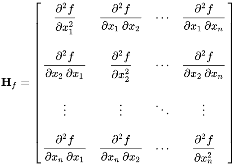
What is Hessian, and how can it be used for faster training? What are its disadvantages?

Hessian Matrix: Uses second-order derivatives for curvature insights, aiding precise optimization and faster convergence.

Faster training with the Hessian:

1. Second-order optimization methods:

• The Hessian can be used in second-order optimization methods, such as Newton’s method or quasi-Newton methods (e.g. BFGS, L-BFGS).

• These methods use the Hessian to compute the update step for the parameters.

• By considering the curvature information, second-order methods can converge faster than first-order methods like gradient descent, especially near the optimum.

2. Adaptive learning rates:

• The Hessian can be used to adapt the learning rates for each parameter individually.

• Methods like AdaHessian and Second-Order Adaptive Learning Rates (SOALR) use the diagonal of the Hessian to scale the learning rates.

• By adapting the learning rates based on the curvature, these methods can accelerate convergence and improve training stability.

3. Curvature-aware optimization:

• The Hessian provides information about the curvature of the loss landscape, indicating the direction and magnitude of the curvature.

• This information can be used to guide the optimization process and make more informed update steps.

• For example, in regions with high curvature, smaller step sizes can be used to avoid can be used to accelerate convergence.

Disadvantage of using the Hessian:

1. Computational complexity: can be computationally expensive, especially for high-dimensional models with a large number of parameters.

2. Memory requirements: storing the full Hessian matrix requires significant memory, especially for large models.

3. Noisy and ill-conditioned Hessian: In some cases, the Hessian matrix can be noisy, especially when the model is far from the optimum or when the data is noisy. Also can lead to unstable updates and hinder convergence.

4. Limited scalability. May not scale well to very large datasets or complex models.

Despite the potential advantages of using the Hessian for faster training, the computational complexity and memory requirements often make it impractical for large-scale deep learning models. First-order optimization methods, such as gradient descent and its variants (e.g., SGD, Adam), remain the most widely used approaches due to their simplicity, scalability, and effectiveness in practice.

Discuss the concept of an adaptive learning rate. Describe adaptive learning methods.

Adaptive learning rate is based on the idea of automatically adjusting the learning rate during the training process to improve the convergence speed and stability of optimization algorithms.

Adam (Adaptive moment estimation)

• Adam combines the ideas from RMSprop and momentum.

• It maintains both the exponentially decaying average of past gradients (first moment) and the exponentially decaying average of past squared gradients (second moment).

• It calculates adaptive learning rates for each parameter.

RMSProp (Root Mean square propagation)

• RMSprop adjusts the learning rate by dividing it by an exponentially decaying average of squared gradients. This method is designed to resolve some of AdaGrad’s issues with rapidly decreasing learning rates.

• RMSprop helps alleviate the problem of learning rates becoming too small and provides a more stable convergence.

AdaGrad (Adpative Gradient)

• Parameters with larger gradients will have smaller learning rates, while parameters with smaller gradients will have larger learning rates. It’s particularly good for dealing with sparse data. However, the learning rates can become very small over time, potentially leading to slow convergence or stagnation.

What is RMSProp and How does it work?

RMSProp: An adaptive learning rate method that adjusts rates based on recent gradient magnitudes.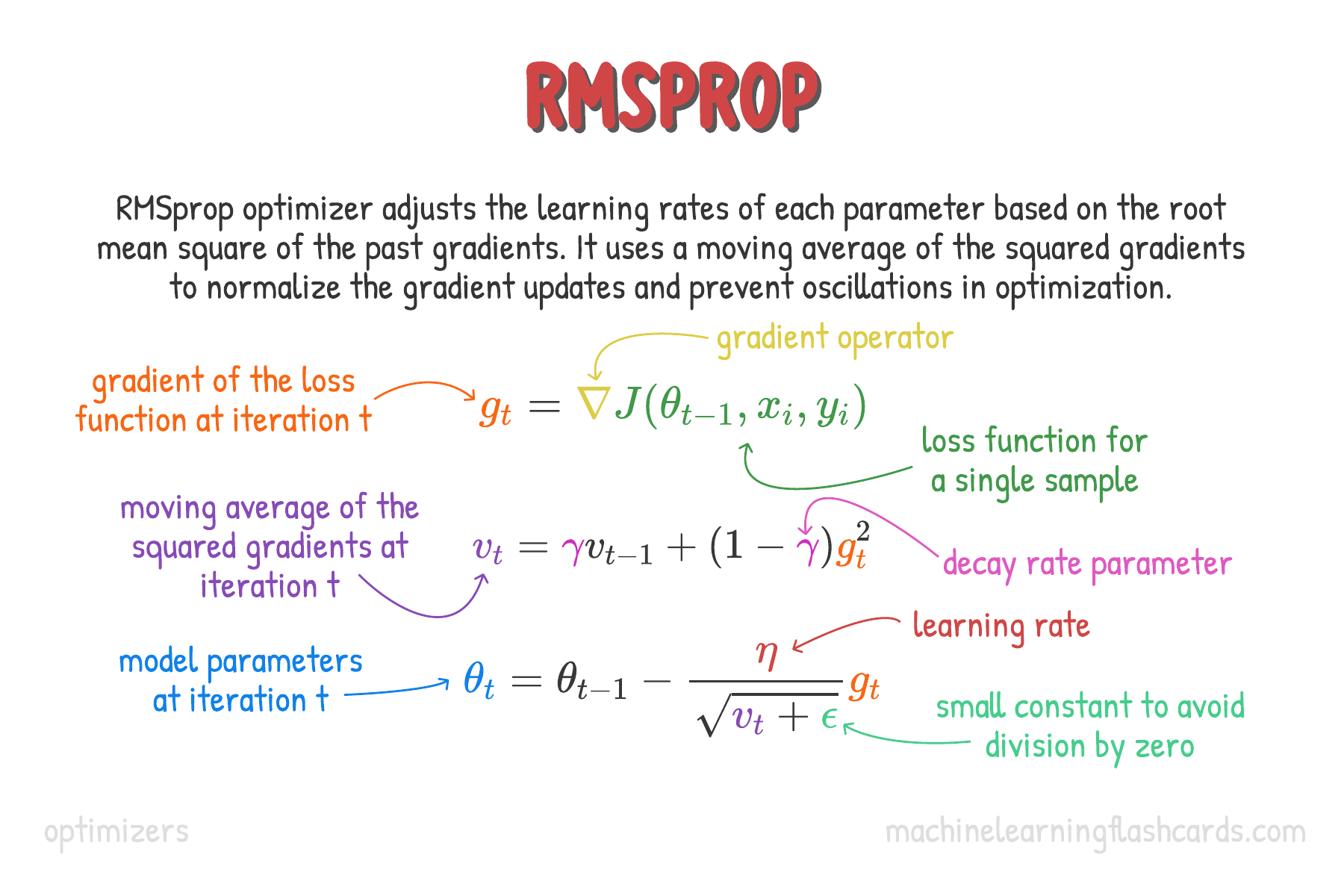

How RMSprop Works

RMSprop works by maintaining a moving average of the squares of gradients and using this average to scale the learning rate for each parameter. This helps in controlling the step sizes, making the optimization process more robust to the choice of learning rate.

1. Calculate the Gradient: At each step, compute the gradient g_t of the loss function with respect to the parameters.

2. Square the Gradient: Compute the square of the gradient g_t ²

3. Update Exponential Weighted Average: Calculate the expontential weighted average of these squared gradients, v_t. This is updated at each step according to the formula.

4. Modify Learning Rate: Adjust the learning rate by dividing it by the square root of v_t. The small constant is added to prevent division by zero and is typically set to a small value, such as 1e-8.

Advantages of RMSprop

• Adaptive Learning Rates: Each parameter gets its own learning rate which makes it possible to make larger or smaller updates depending on their importance and frequency.

• Convergence Improvement: By adapting learning rates, RMSprop can converge faster than conventional gradient descent, especially in contexts involving noisy or sparse gradients.

• Robustness: The method is less sensitive to the initial learning rate and hyperparameter settings compared to simple momentum and AdaGrad.

What is Adam and why is it used most of the time in NNs?

Adam is an optimization algorithm that combines the best properties of the AdaGrad and RMSprop algorithms to provide an efficient solution for training neural networks.

How Adam Works

Adam maintains both the first moments (the mean) and the second moments (the uncentered variance) of the gradients, using these to adapt the learning rate for each parameter during training.

1. Calculate the Gradient: At each step, compute the gradient gt​ of the loss function with respect to the parameters.

2. Update First Moment (mean): Update the biased first moment estimate, mt​, which is the exponential moving average of the gradients:

   mt​=β1​mt−1​+(1−β1​)gt, where β1​ is typically around 0.9.

3. ​Update Second Moment (uncentered variance): Update the biased second moment estimate, vt​, which is the exponential moving average of the squared gradients: vt​=β2​vt−1​+(1−β2​)gt² ​, where β2​ is typically around 0.999.

4. Correct Moments: Since both mt​ and vt​ are biased towards zero, especially during the initial time steps, they are corrected by dividing them by 1−β1t​ and 1−β2t​ respectively.

5. Update Parameters: Adjust the parameters using the corrected estimates:

   θt+1​=θt​−v^t​​+ϵη​m^t​

   Here, η is the learning rate, and ϵ is a small constant (e.g., 10−810−8) to prevent division by zero.