Chapter 6: Roots (Open Methods)

true

(T/F) open methods require only a single starting value or two starting values that do not necessarily bracket the root

true

(T/F) open methods sometimes diverge or move away from the true root

- fixed point iteration
- Newton- Raphson
- Secant
- Modified Secant

open methods include

utilizing fixed point iteration(one point / successive substitution) to get x on the left hand side.

for more on fixed point refer to lecture powerpoint

how do open methods predict a root?

bisection and secant method. It's good because it combines them

Fzero uses

- allows one to predict a new value of x as a function of an old value of x

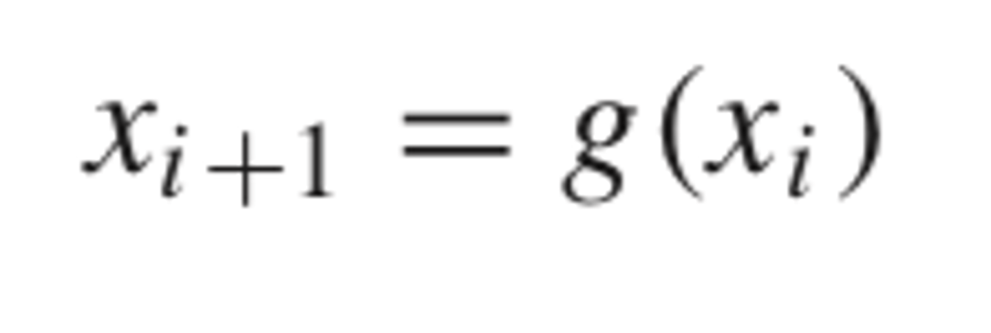
Thus, given an initial guess at the root xi , Eq. (6.1) can be used to compute a new estimate xi+1 as expressed by the iterative formula

& so on

x(i+2) = g(x(i + 1))

what is the advantage of fixed point iteration?

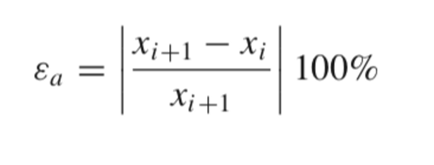
approximate relative error is given by this formula

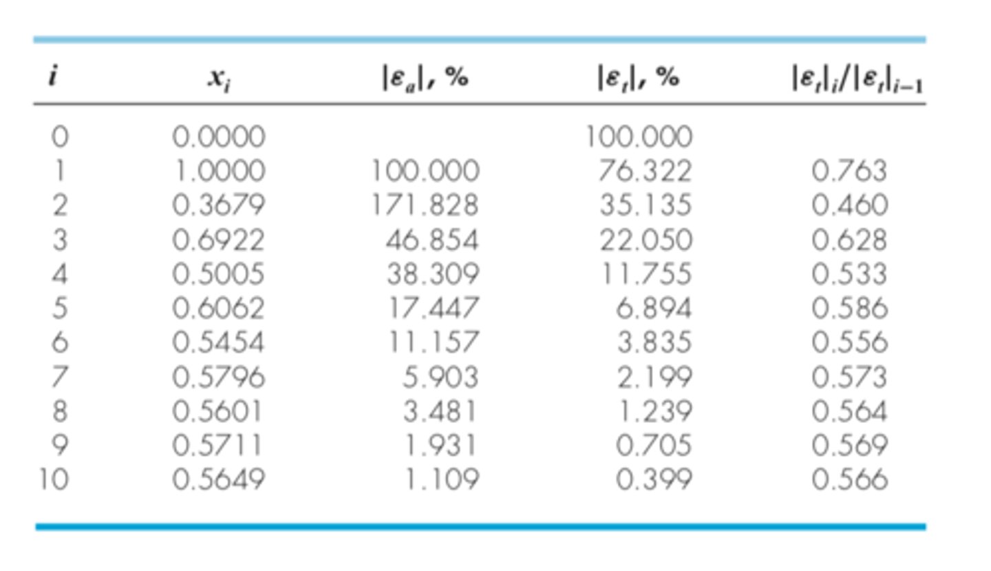
the approximate percent relative error is halved after each iteration

fixed point iteration has linear convergence and can be proved by

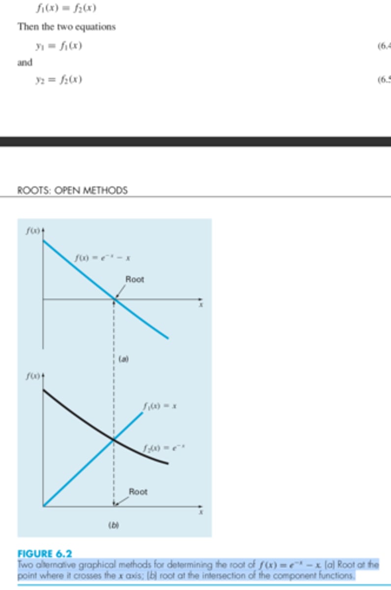
- separating the equation into two components and then graphing the components separately and seeing where they intersect.

- just graph the original function and see where it intersects the x axis

two alternative graphical methods for determining the root of an equation are

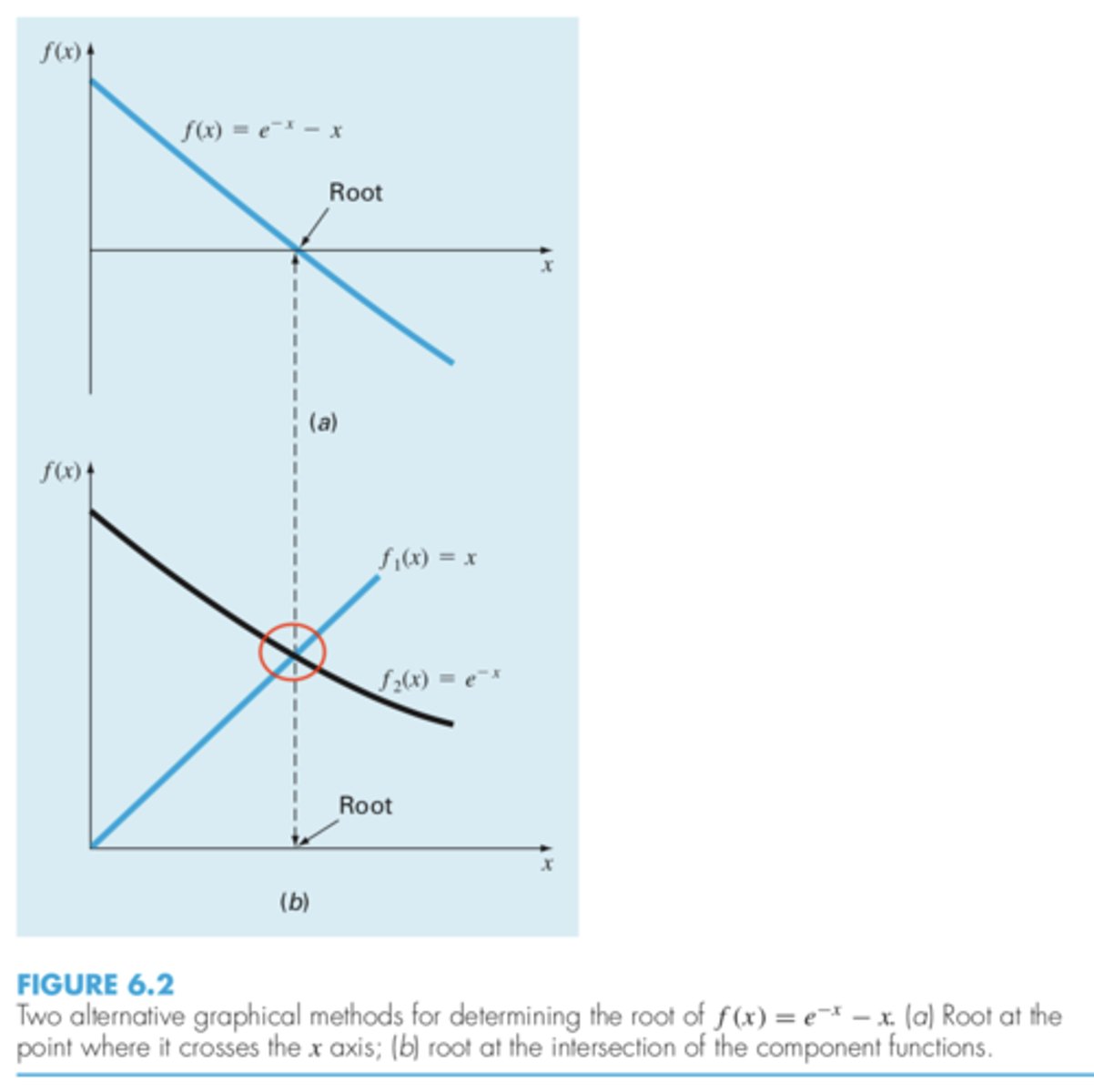
the intersection of the two components of the equation (it's the same thing as the root of the function) (denoted by red circle)

-- idk if abscissa will always be the root!

what is an abscissa

For the first case (Fig. 6.3a), the initial guess of x0 is used to determine the corresponding point on the y2 curve [x0, g(x0)]. The point [x1, x1] is located by moving left horizontally to the y1 curve. These movements are equivalent to the first iteration of the fixed-point method:
x1 = g(x0)
Thus, in both the equation and in the plot, a starting value of x0 is used to obtain an esti- mate of x1. The next iteration consists of moving to [x1, g(x1)] and then to [x2, x2].

fixed point iteration graphically

|g′(x)| < 1.

Convergence for fixed point iteration occurs when

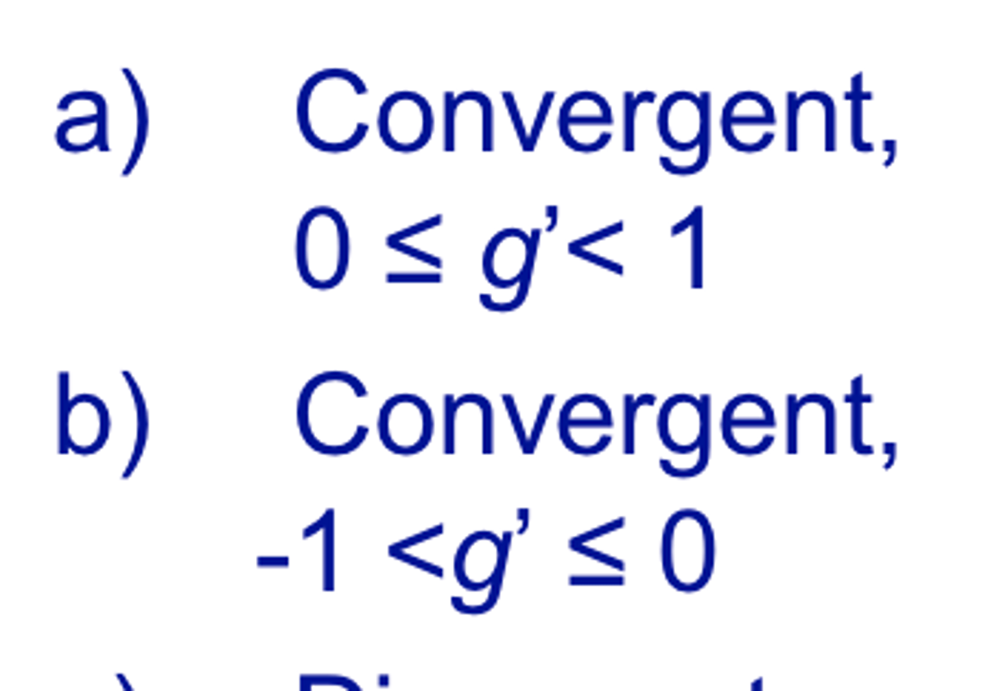
fixed point iteration convergence

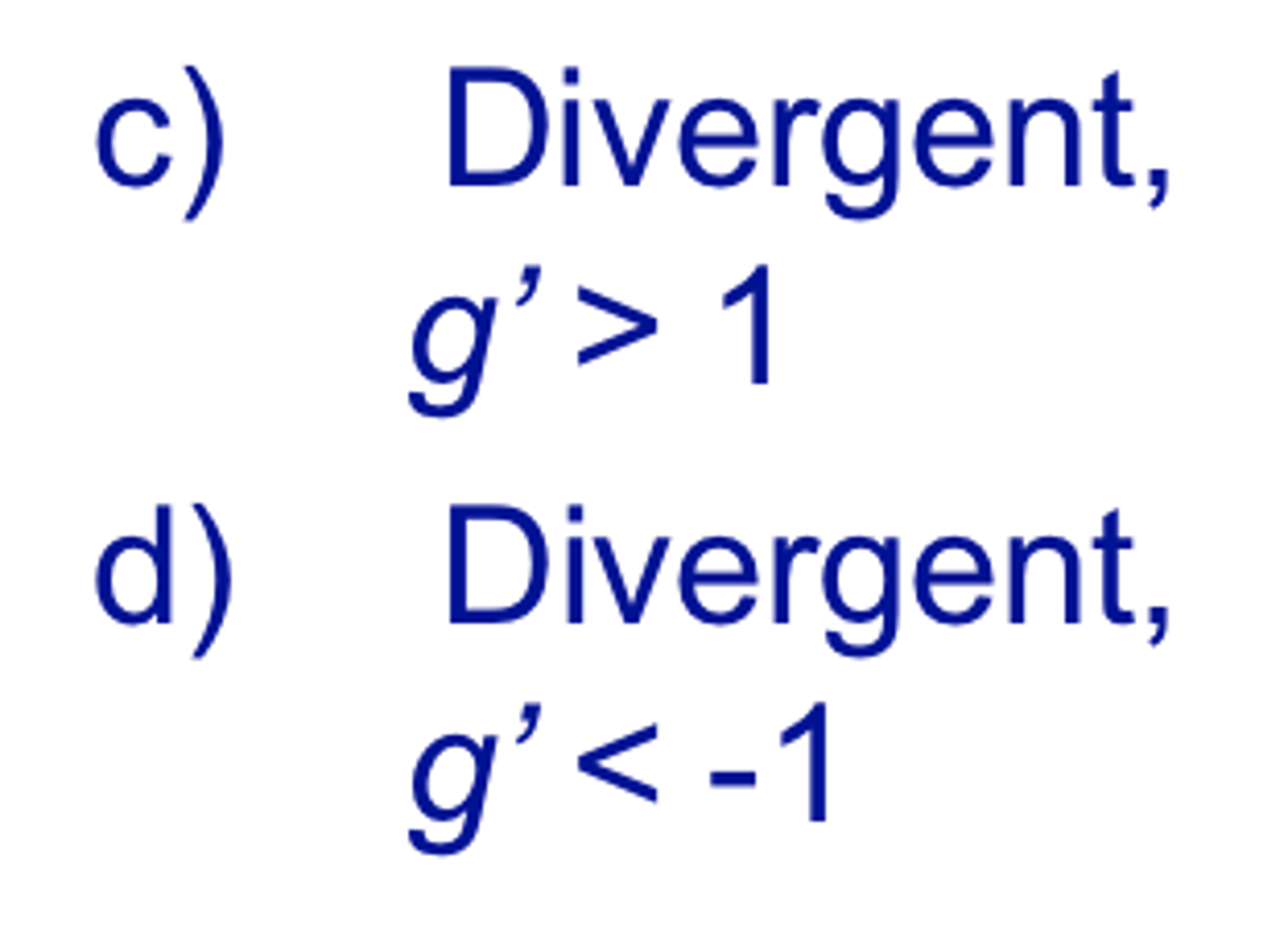
fixed point iteration divergence

decrease with each iteration

for fixed point iteration, if |g′| < 1 , the errors

grow

for fixed point iteration, if |g′| > 1, the error

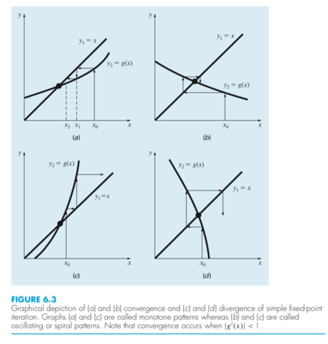
positive, and hence the errors will have the same sign (a and c)

If for fixed point iteration, the derivative is positive, the errors will be

change sign on each iteration (b and d)

If for fixed point iteration, the derivative is negative, the errors will

if the initial guess of the root is xi , a tangent can be extended from the point [xi , f (xi )]. The point where this tangent crosses the x axis usually represents an improved estimate of the root.

Newton Raphson method

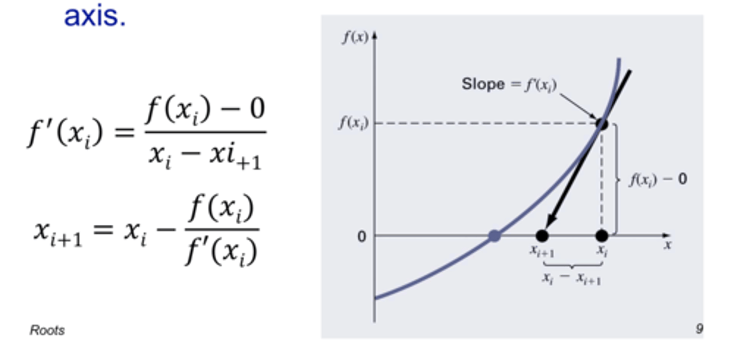
for the newton raphson method, The first derivative at x is equivalent to the slope ... which can be rearranged to ..

no. Well, the percent relative error at each iteration decreases much faster for newton than fixed

usually is the fixed point iterative method faster than the newton raphson method?

proportional to the square

for newton raphson method, the error should be roughly ..... of the previous error

NOTE: the number of significant figures of accuracy approximately doubles with each iteration

is exhibited by newton raphson method because the error is roughly proportional to the square of the previous error... this means the number of significant figures of accuracy approximately doubles with each iteration

quadratic convergence

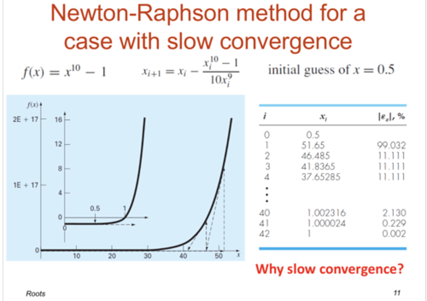
example of slow convergence using newton raphson method

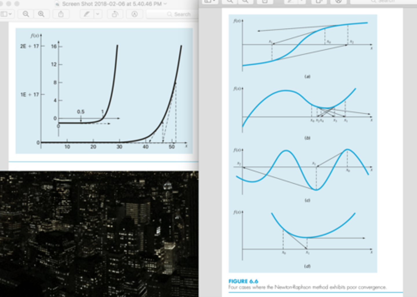
* multiple roots

when the first guess is in a region where the slope is near zero (so first iteration flings solution far away!! so it takes time to converge back in on it (nature of the function basically*) -- figure on left

* (figure a) inflection point (f'(x) = 0) occurs in the vicinity of a root, causing the iterations to diverge from the root. So slow when root is at an inflection point

* (figure b) illustrates the tendency of the Newton-Raphson technique to oscillate around a local maximum or minimum. Such oscillations may persist, or, as in Fig. 6.6b, a near-zero slope is reached whereupon the solution is sent far from the area of interest.

* (fig C) encountering near zero slopes (disaster cause a derivative of 0 causes division by 0)

* (fig d) tangent line shoots off horizontally. never hitting the x axis

when is there slow convergence for newton raphson method? (4)

true. its convergence depends on the nature of the function and on the accuracy of the initial guess.

(T/F) There is no general convergence criterion for Newton-Raphson

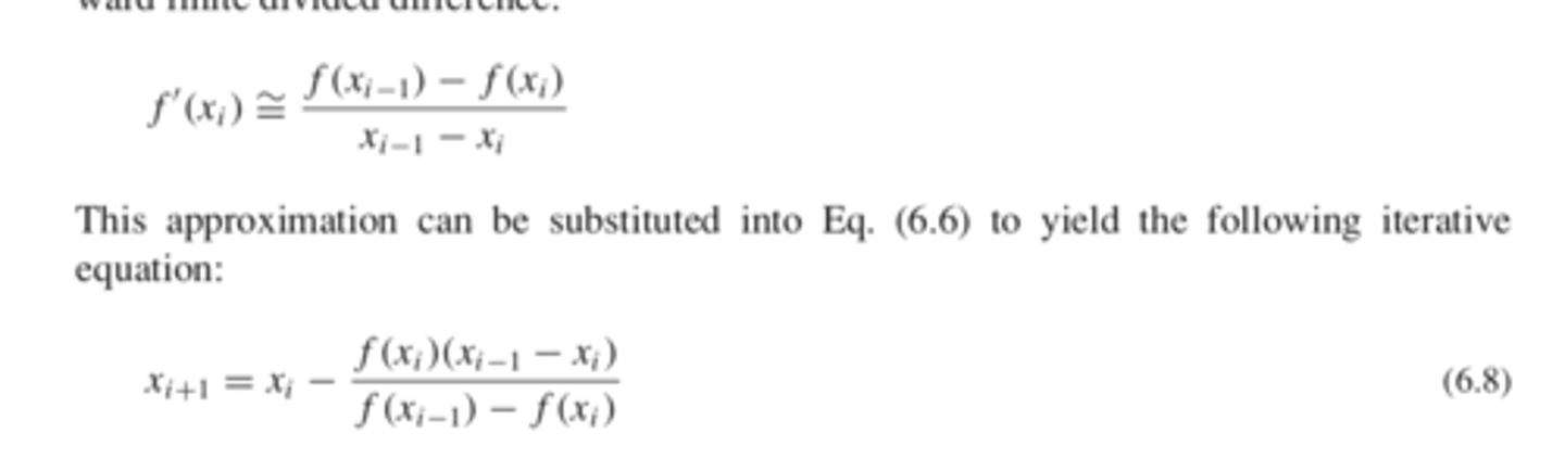
when derivatives are hard to evaluate, so use the backward finitde divided difference

when can the secant method be used?

uses the finite divided difference and two arbitrary initial guesses

used when derivatives are hard to evaluate

secant method

because f(x) is not required to change signs between the estimates

why is the secant method not considered a bracketing method?

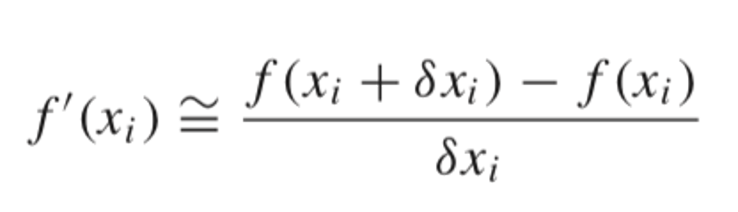
a fractional perturbation of the independent variable to estimate f'(x)

where sigma is a small perturbation fraction.

instead of using arbitrary initial guesses for the secant method, what can you do

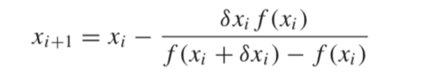
a small perturbation fraction is used instead of two arbitrary initial guesses

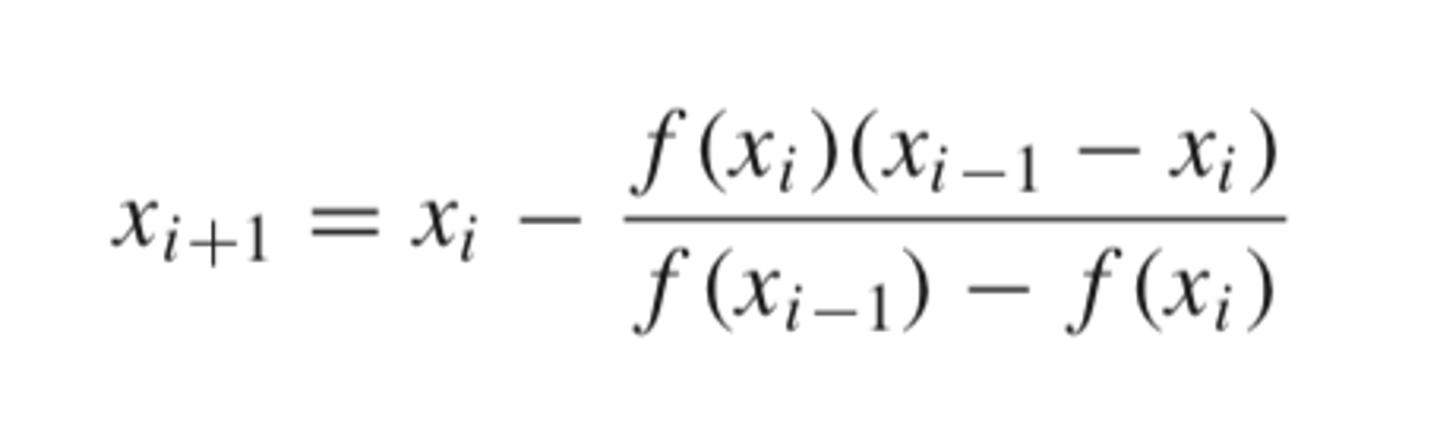
modified secant method

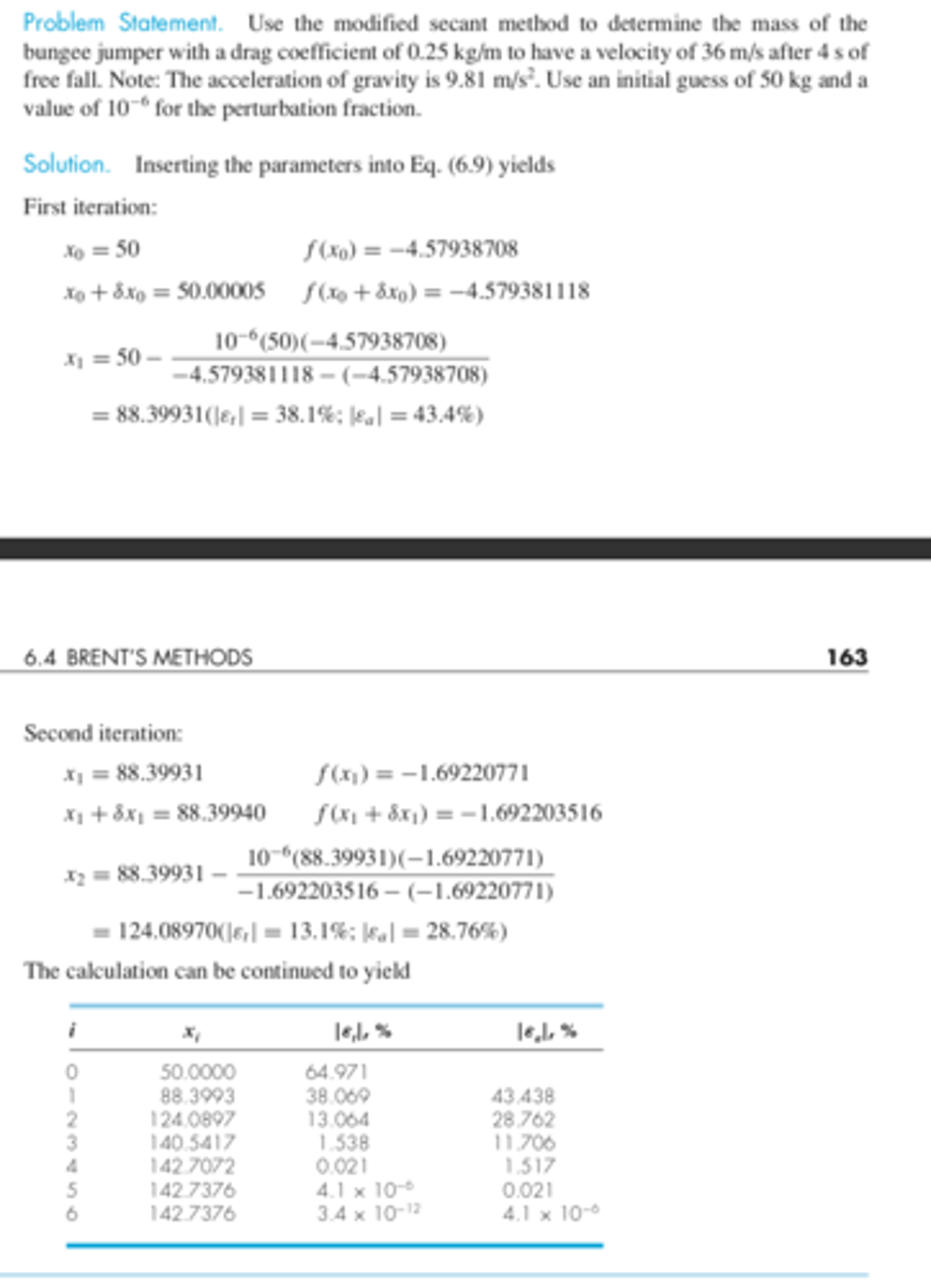
modified secant method example

the perturbation might not be a proper value. It sigma is too small, the method can be swamped by round-off error caused by subtractive cancellation in the denominator of Eq. (6.9). If it is too big, the technique can become inefficient and even divergent. How- ever, if chosen correctly, it provides a nice alternative for cases where evaluating the derivative is difficult and developing two initial guesses is inconvenient.

what are possible errors that come with the modified secant method

hybrid approach that combined the reliability of bracketing with the speed of the open methods

chooses when to use which

didn't read this section (6.4) page 163

brent's mehod

used to find the real root of a single equation.

takes in the function and an initial guess (open method)

or two guesses in a vector can also be passed.


(another card tells you more specifics)

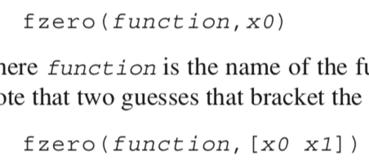
fzero()

the guess that you need to pass needs to be a guess near the root. for example x^2 - 9 has two roots, so if you pass 0 it'll give you -3, if you pass 4, 3.

for fzero function, wat is a disadvantage,

it first performs a search to identify a sign change. This search differs from the incremental search described in Section 5.3.1, in that the search starts at the single initial guess and then takes increasingly bigger steps in both the positive and negative directions until a sign change is detected.

Then it does the fast methods (secant and inverse quadratic interpolation) unless an unacceptable result occurs (root estimate falls outside bracket), then bracketing method occurs.

once it finds an acceptable root (or gets closer to the root) it switches to the faster methods. Bisection typically dominates at first, but then switches to the other

how does the fzero function work if a single initial guess is passed,

secant and inverse quadratic interpolation

fast root finding methods

[x,fx] = a vector containing the root x and the function evaluated at the root fx, options is a data structure created by the optimset function, and p1, p2... are any parameters that the function requires. Note that if you desire to pass in parameters but not use the options, pass an empty vector [] in its place.

fzero syntax

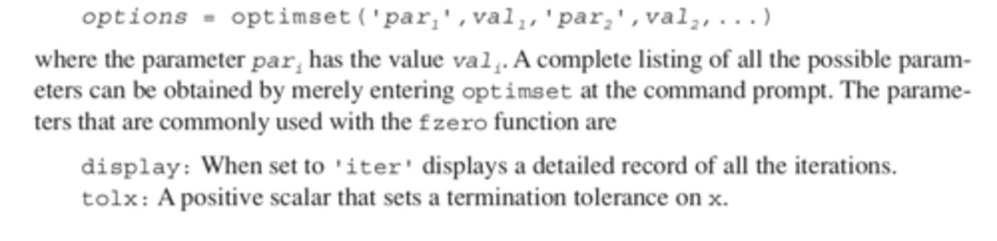
optimest function spills out all the data that occurred during the fzero function

bisection method and newton raphson method

for polynomials, which root finding method is utile for finding a single root

roots function

if we want to find all the roots of a polynomial, what do we use

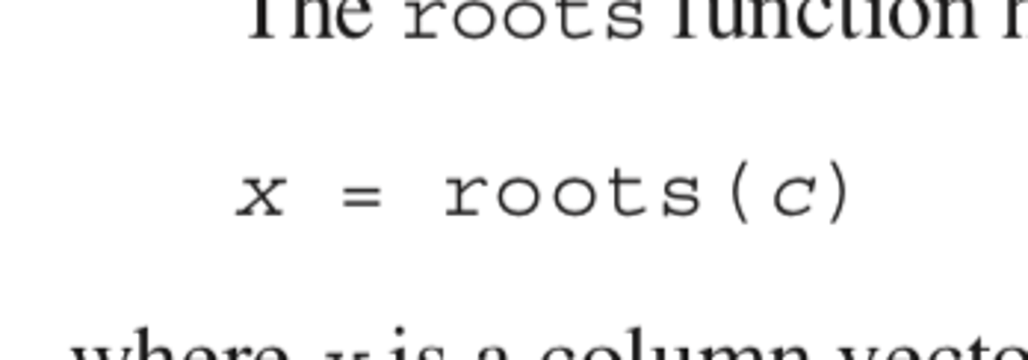
x is a column vector containing the roots and c is a row vector containing the polynomial coefficients

roots function syntax

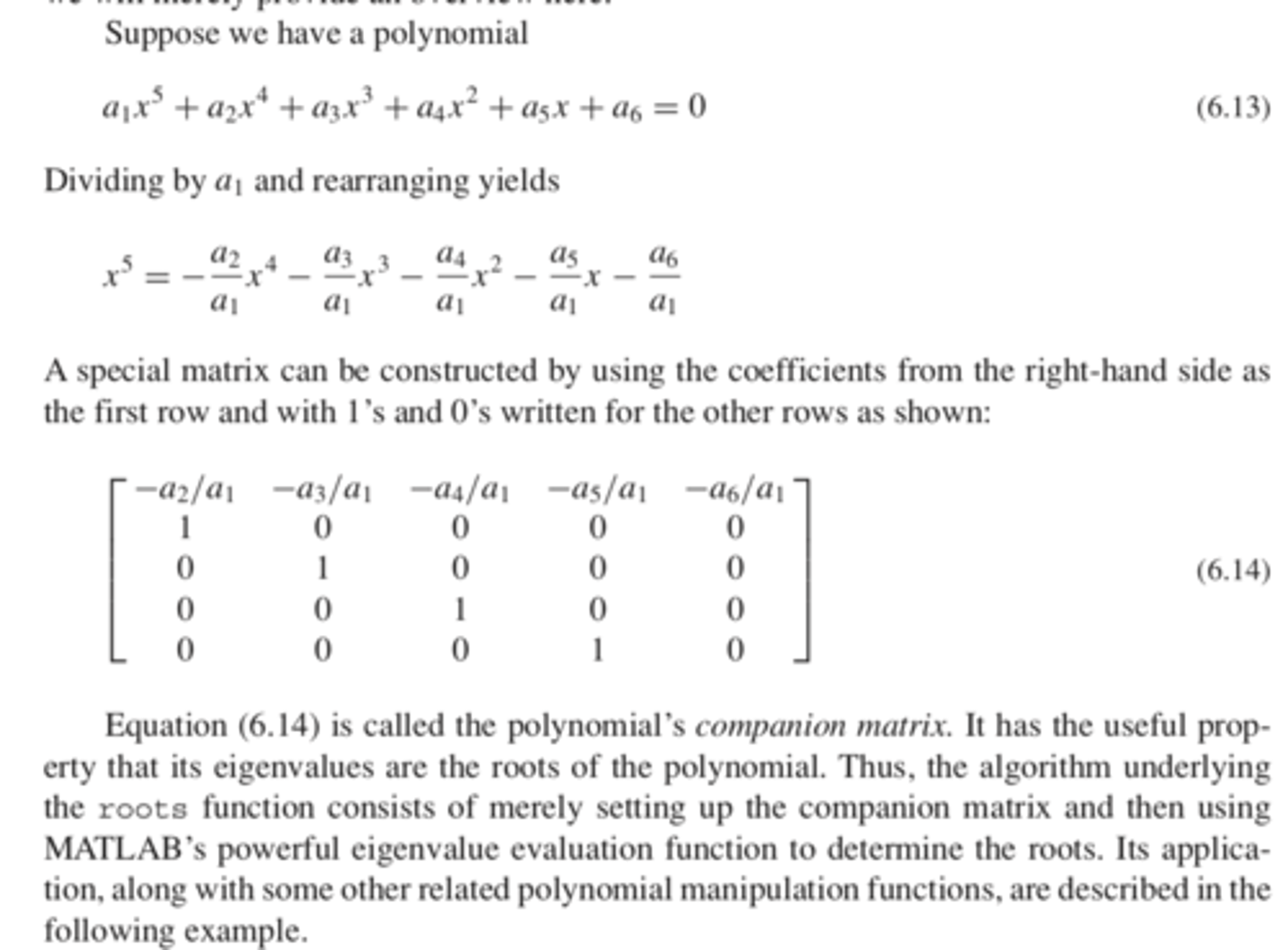
treats it as an eigenvalue problem

creates a companion matrix by dividing the all the coefficients by the first coefficient then placing them in a matrix with 1s and 0s. The companion matrix has a useful property that its eigenvalues are the roots of the polynomial.

after it makes the matrix, it uses matlab's eigenvalue evaluation function to determine the roots of the polynomial.

how does the roots function work

poly() function

inverse function of roots function is

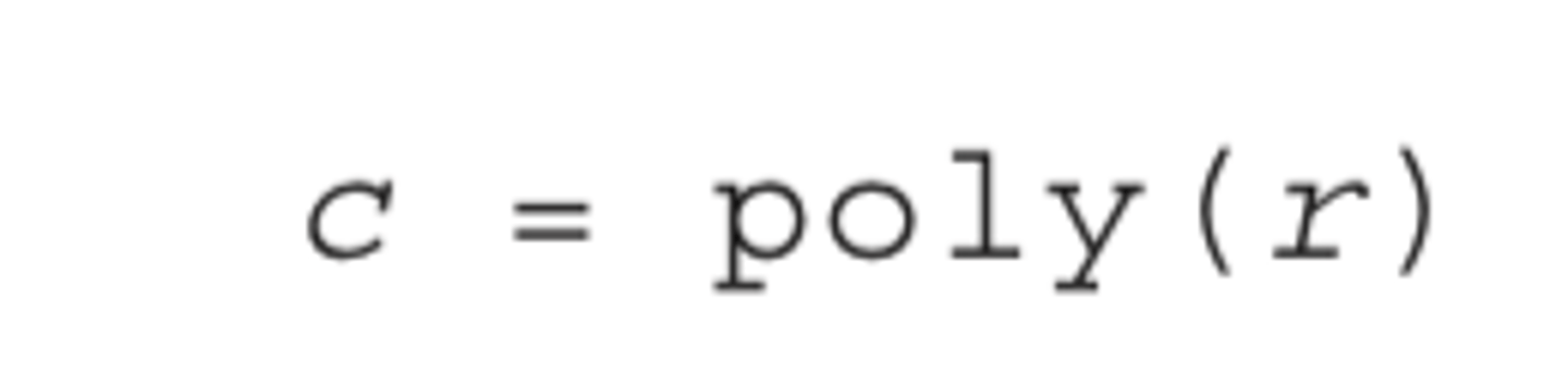
when passed the values of the roots, it returns the polynomial's coefficients.

where r is a column vector containing the roots and c is a row vector containing the polynomial's coefficients.

poly() function

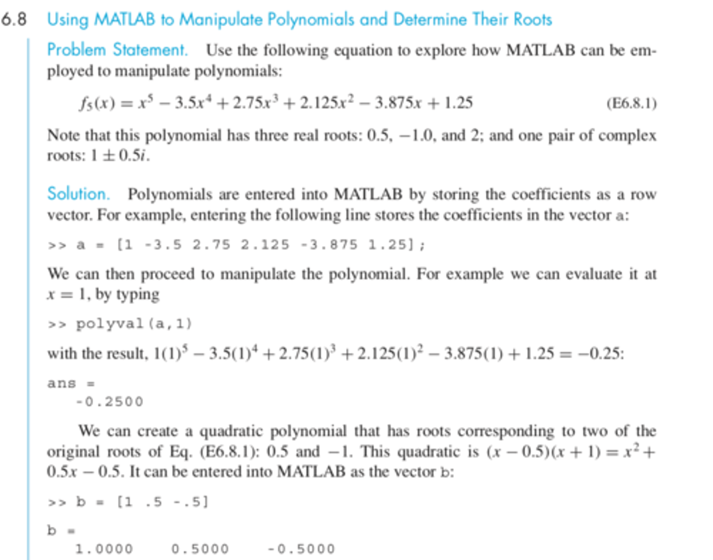
example, finding roots of polynomial. using polyval(), poly(), roots(), and deconv()

(1/3)

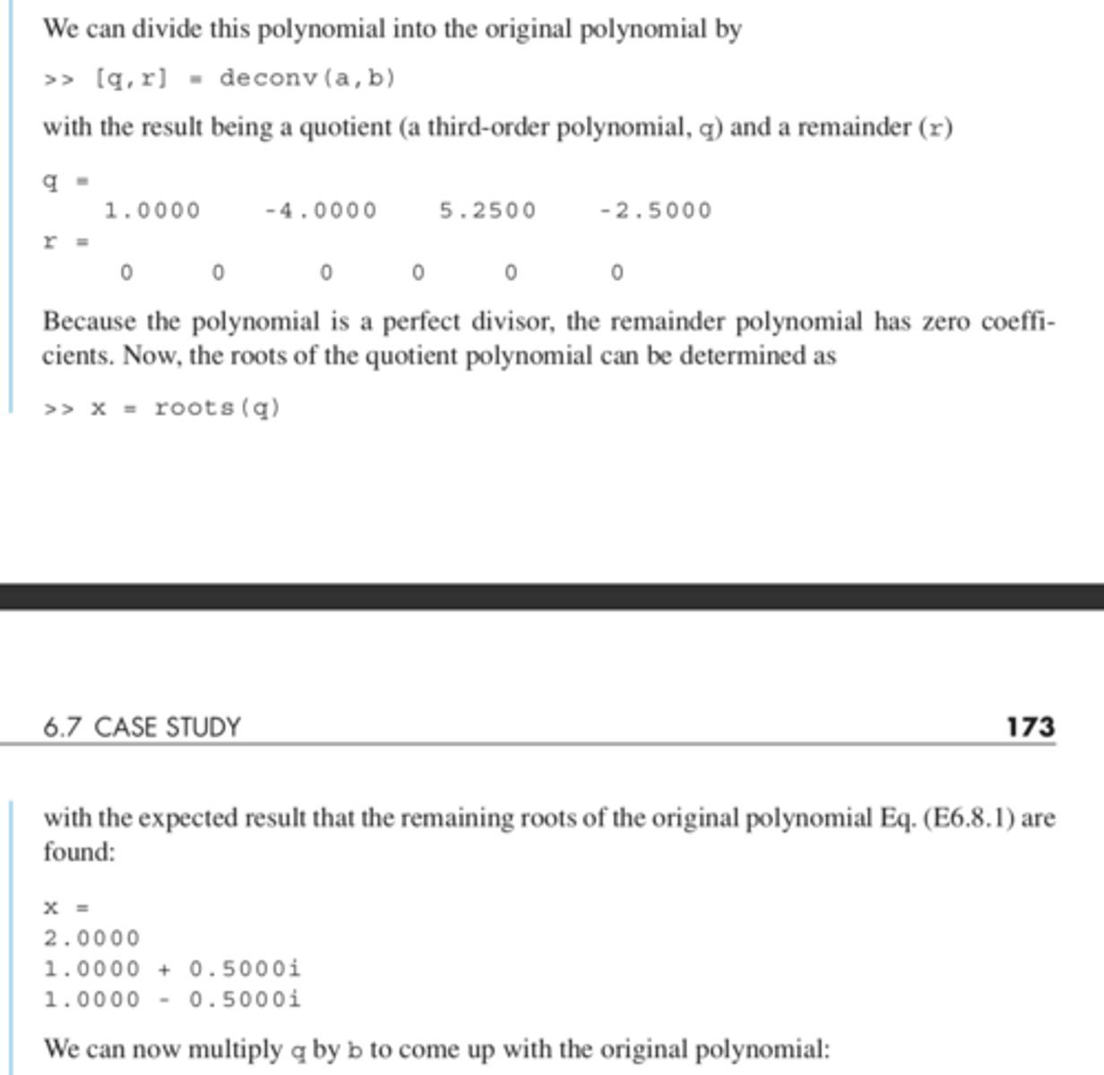
(2/3)

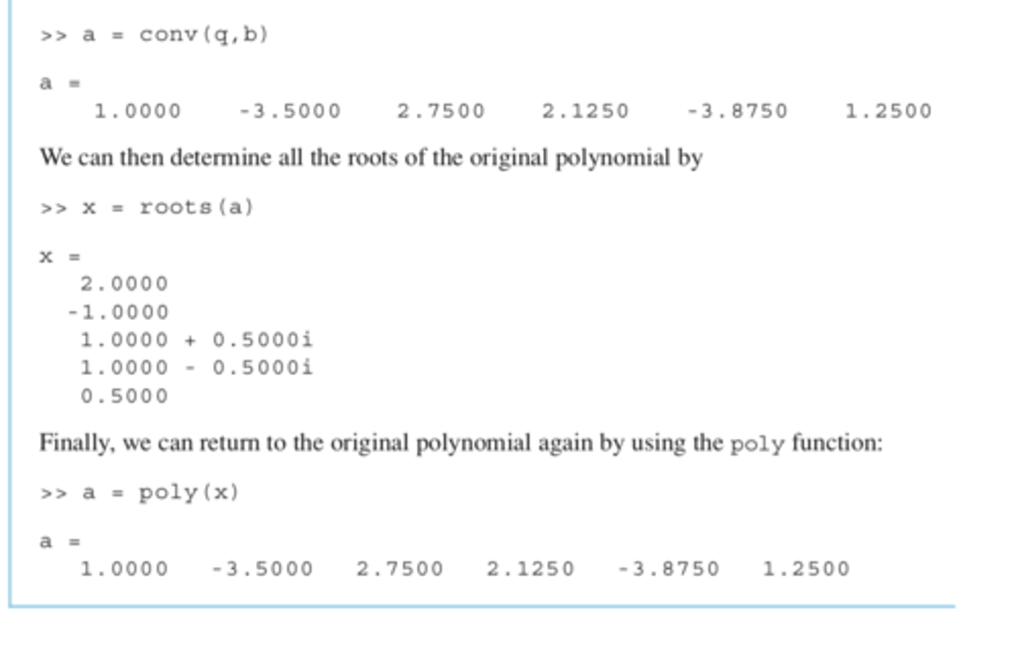
(3/3)

- combines reliability of bracketing with speed of open methods.

- chooses when to do which.

for bracketing method uses bisection and for open methods uses secant method or inverse quadratic interpolation

Brent's method

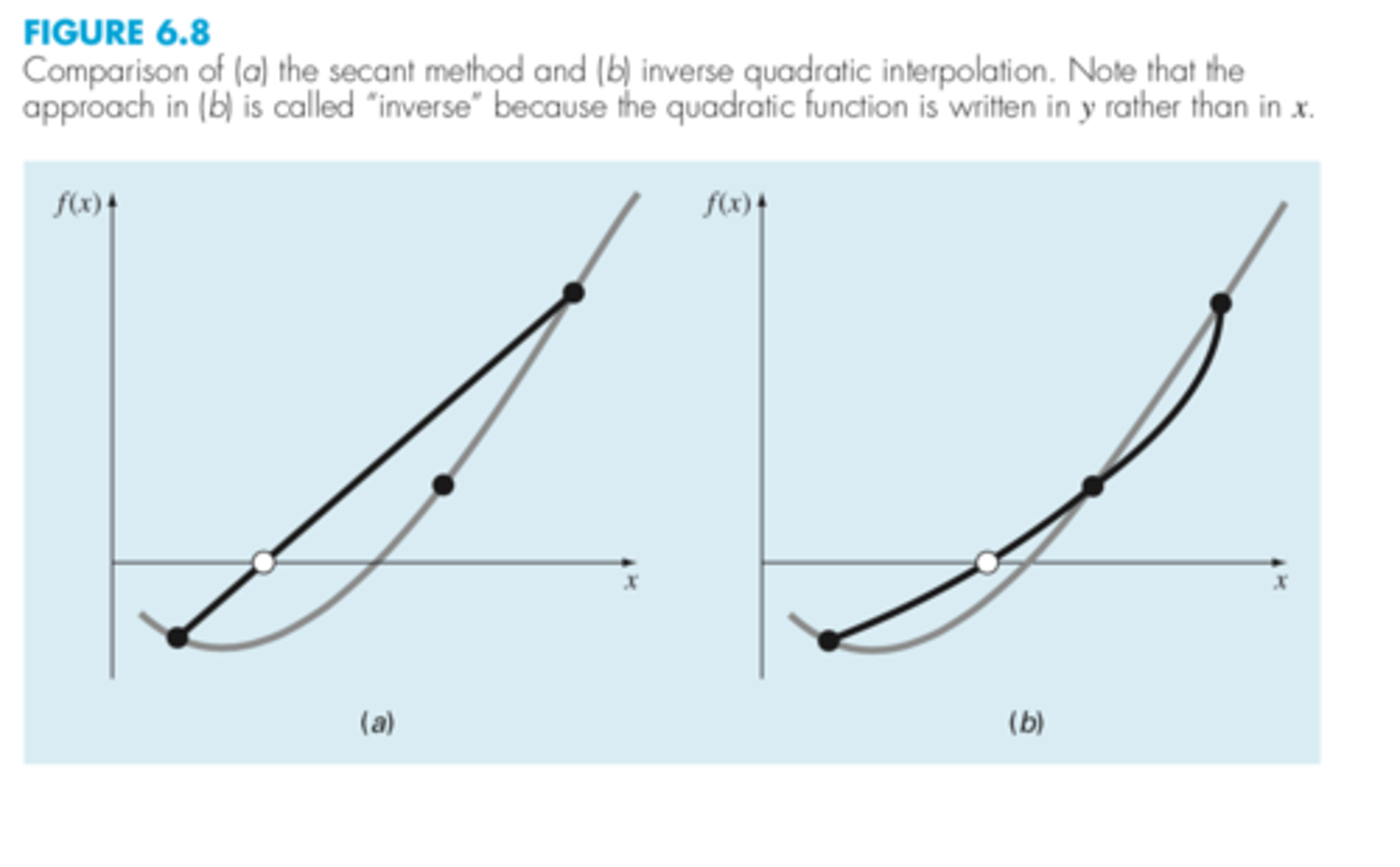
secant method is sometimes referred to as such because the lines that connects the two guesses is used to estimate the new root estimate by observing where it crosses the x axis

linear interpolation method

determining a sideways quadratic function that goes through 3 points and observing where it intersects the x axis
the point where it intersects the x axis will be used as the new root estimate

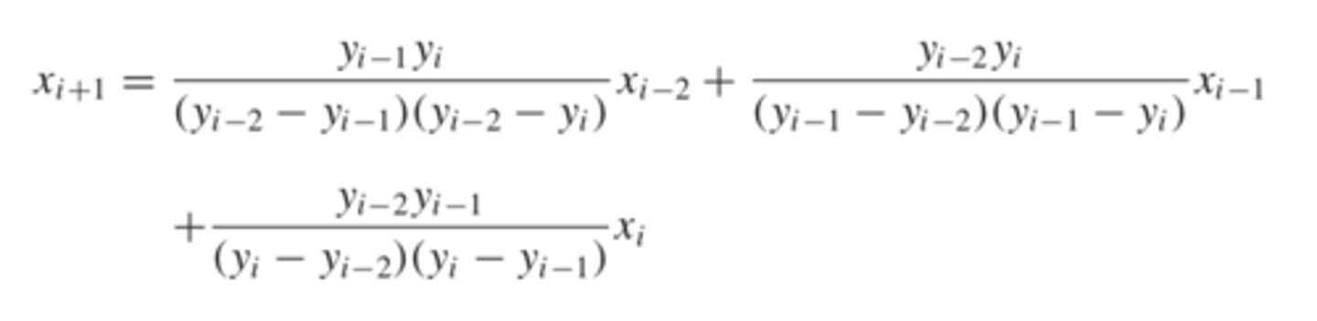
y = 0 corresponds to the root x(i+1)

this equation finds the root

inverse quadratic interpolation

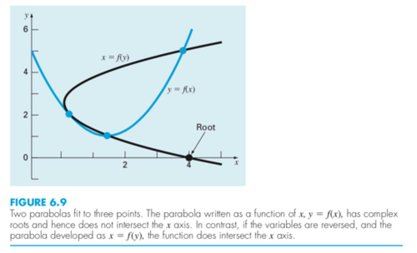
the parabola might not intersect the x axis (when the parabola has complex roots)

so inverse quadratic interpolation was created to switch the axis and make a sideways graph

what is the flaw with quadratic interpolation not inverse

inverse quadratic interpolation is better as seen in the picture

comparing inverse quadratic interpolation vs secant

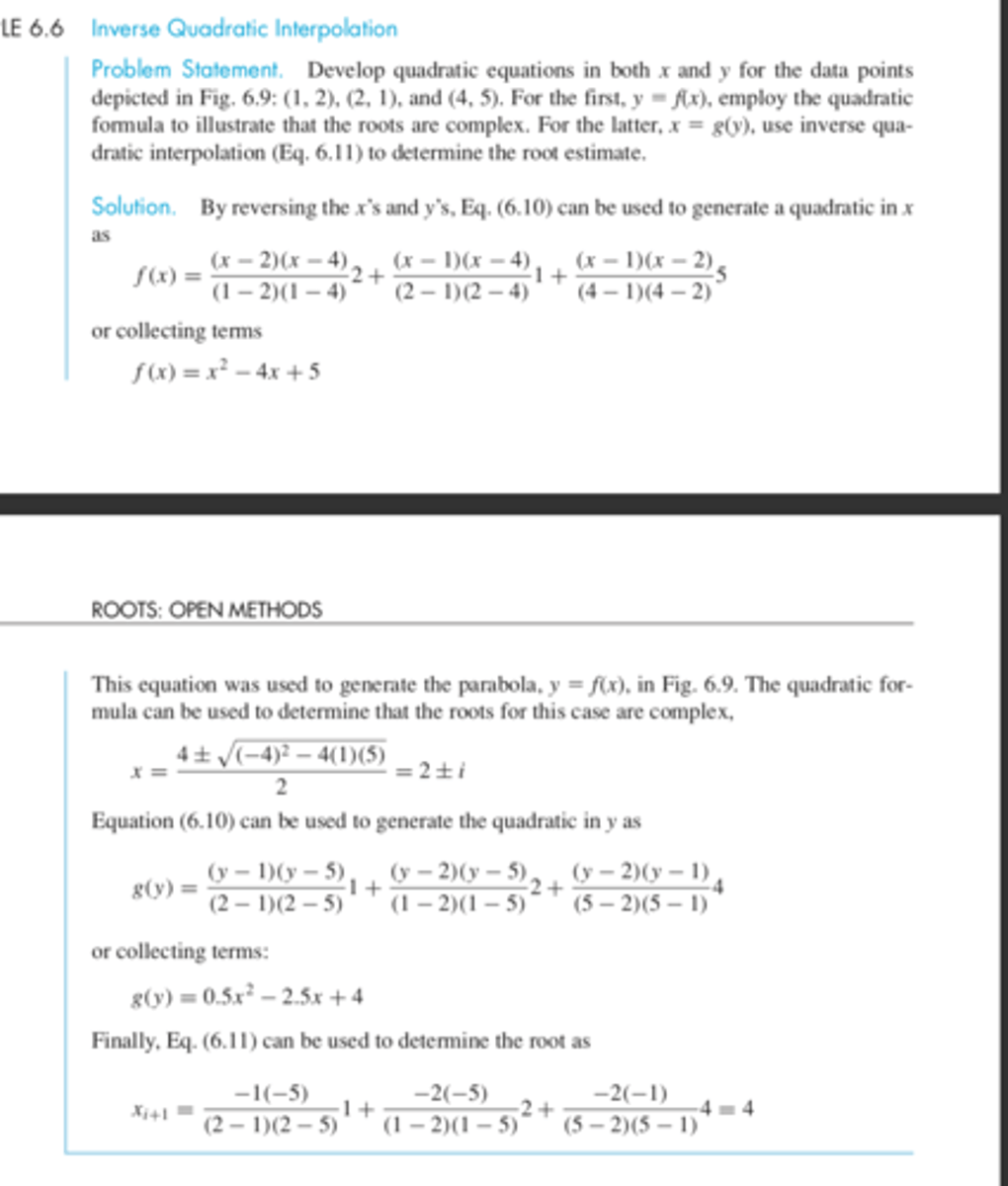
inverse quadratic interpolation example

reversing x and y in this equation will yield a quadratic in x

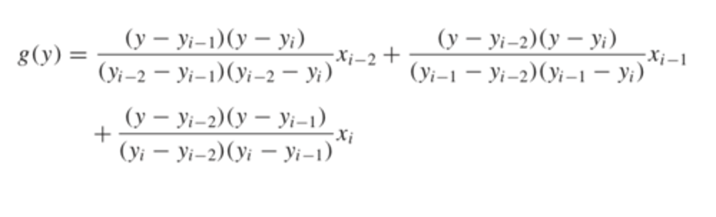
quadratic in y is made using this equation

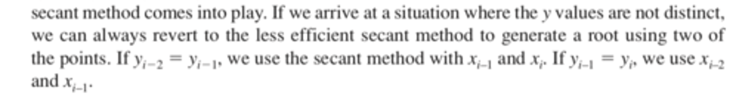
If the three y values are not distinct (i.e., yi-2 = yi-1 or yi-1 = yi), an inverse quadratic function does not exist.

If we arrive at a situation where the y values are not distinct, we can always revert to the less efficient secant method to generate a root using two of the points. If yi 2 yi 1, we use the secant method with xi-1 and xi. If yi-1 yi, we use xi-2 and xi-1.

when does inverse quadratic interpolation not work