time series

switching model

dynamic behavior of a series (mean, variance) changes depending on the state (or regime) the world is in at time t

TAR/MSW

In a TAR (Threshold AR) model, the regime is observable and determined by a threshold variable qt crossing a value c. In a MSW (Markov-Switching) model, the regime is unobservable (latent) and determined by a probability (Markov process)

Markov property

assumption that the current regime St depends only on the previous period st-1 and not the entire past, memory less process

transition matrix

maxtrix P containing conditional propabilities of switching from a regime to another , or staying in the same one , the sum of probilities from a given regime must be equal to 1

SETAR

The SETAR is a threshold model where the regime switch is triggered by the series' own past values,You cannot use standard mathematical equations (derivatives) because the switch is abrupt. You must perform a grid search (testing many possible thresholds) to find the best one

What problem(s) may arise if the standard AIC and SIC information criteria were applied to the determination of the orders of each equation in a TAR model? How do suitably modified criteria overcome this problem?

• nsufficient Penalty: Standard criteria (AIC/SIC) applied naively may not correctly penalize the estimation of additional TAR-specific parameters, such as the threshold c and delay d. This often leads to overfitting (selecting overly high orders p_1, p_2).

• Sample Size: If criteria are applied separately to each regime, the sample sizes (T_1, T_2) are random and can be too small, making estimation unstable.

• solution modifed criteria

e) A researcher estimates a SETAR model with one threshold and three lags in both regimes. He then estimates a linear AR(3) model and proceeds to use a likelihood ratio test to determine whether the non-linear threshold model is necessary. Explain the flaw in this approach.

The problem is that the threshold parameter c is unidentified under the null hypothesis of linearity (H_0). If the model is truly linear, the threshold does not exist or is irrelevant, as the coefficients are the same everywhere, One must use critical values obtained via simulation (like the SupF test) rather than standard statistical tables

ARCH(q) VS GARCH(p,q)

EN: The ARCH model makes today's volatility depend on past squared errors. The GARCH model adds past volatility as an explanatory variable. GARCH is better because it is more parsimonious (fewer parameters)

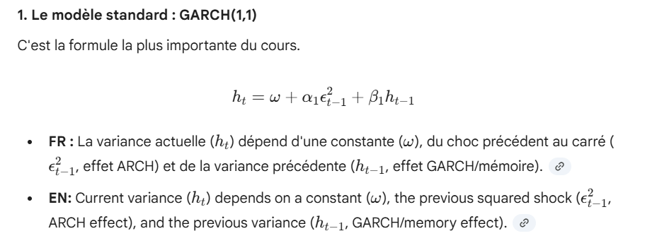
GARCH(1,1)

EN: This is the industry standard model. It is usually sufficient to capture financial volatility persistence.,

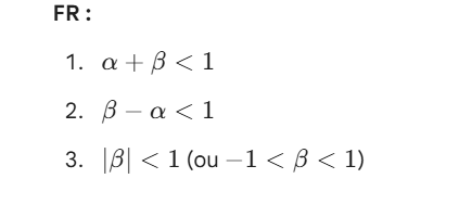
alpha1+beta1<1 plus la somme proche de 1, plus la volatilité met du temps à revenir à la normale.

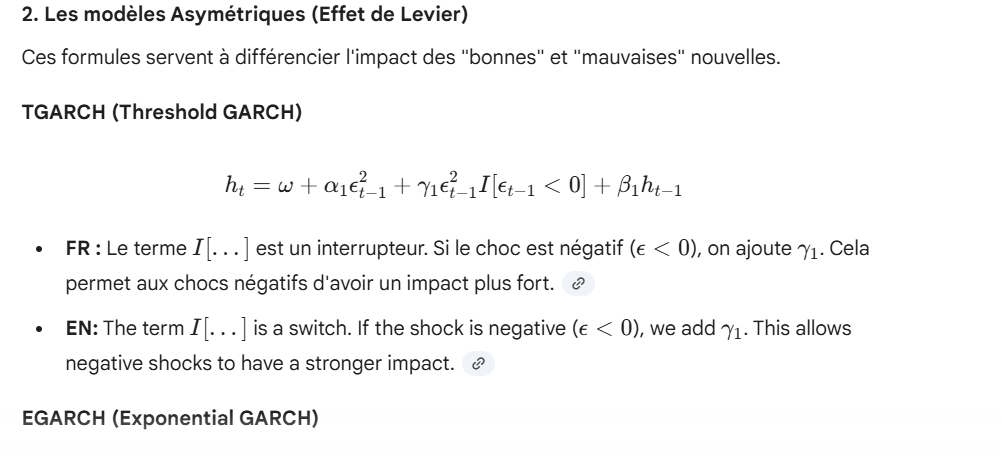
leverage effect

EN: Financial markets are asymmetric: bad news (negative shocks) increases volatility more than good news. Standard GARCH (symmetric) misses this,EN: To capture this leverage effect, we use EGARCH (using log variance) or TGARCH (using a threshold at 0 to distinguish positive/negative shocks)

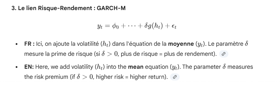
GARCH-M

EN: Financial theory states: "Higher risk = Higher expected return". GARCH-M includes volatility directly in the mean equation to test for this risk premium.

QML volatilité

EN: Financial returns are not Normally distributed (fat tails). We use the QML method for estimation because it remains robust even if the distribution is not Normal

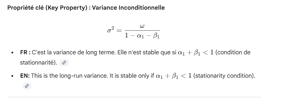
unconditional variance

long run variance

egarch

diagnostical checking garch

EN : We don't look at raw errors, but errors divided by estimated volatility: {z}_t = \epsilon}_t / \sqrt{h}}, white noi moyenne 0 variance 1

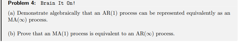
AR, MA

AR (AutoRegressive): y_t depends on its own past values (y_{t-1}). "Memory of the level"

MA (Moving Average): y_t depends on past errors epsilon_{t-1}). "Memory of shocks"

stationnary

series is stationary if its mean and variance are constant over time. If it has a trend (unit root), it is non-stationary and must be differenced (d$times)

the series eventually reverts to its mean (mean-reverting behavior). This is the opposite of a non-stationary series (like a random walk) where the shock has a permanent effect Here is transitory shock

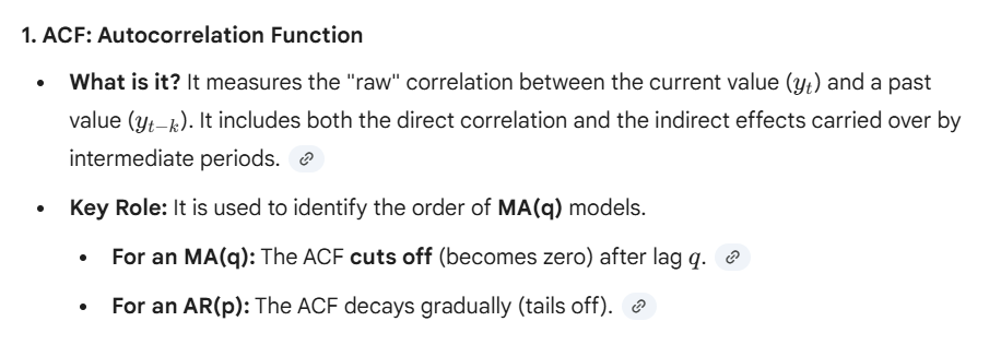
ACF

Autocorrelation Function

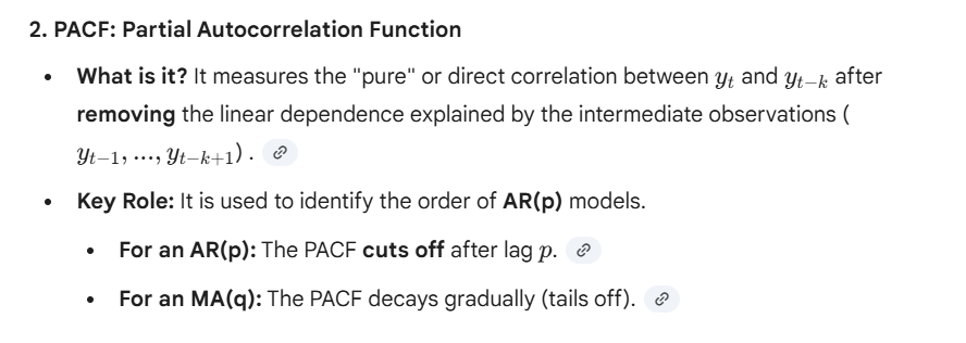
PACF

Partial Autocorrelation Function

determinist/stochastic

• Deterministic (D=0): The pattern is stable over time. We use Dummy variables

• Stochastic (D=1): The pattern changes over time. We use seasonal differencing (Delta_S)

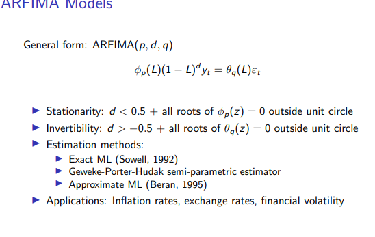
arfima

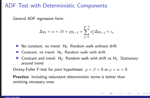
adf test

• For ADF, we want to reject H_0 (p-value < 0.05) to prove stationarity.

• For KPSS, we want to keep H_0 (p-value > 0.05) to claim stationarity.

MA , AR

Short memory. After q steps, the forecast goes flat to the mean (0). Long memory. The forecast reverts to the mean slowly (asymptotically).

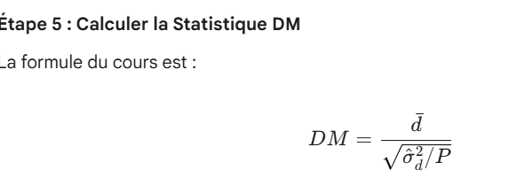
stat de test

le term phi

VA de phi1 dans close to 0 (e.g., 0.2): Low persistence. The series reverts to the mean very quickly after a shock.,

close to 1 (e.g., 0.95 or 0.99): High persistence. It is technically stationary (since $<1$), but the shock takes a very long time to disappear.

$\phi_1 = 1$: Unit root (Random Walk). The shock is permanent. Non-stationary.

Ar stationnary conditions

Ma c’est toujours stationnaire

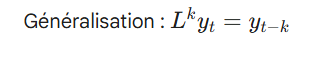
lag error operator

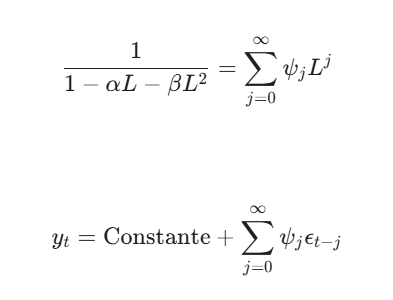
theoreme de wold

ar stationnary

AR processes are stationary only conditional on their characteristic roots lying outside the unit circle

probleme non statio

• Spurious Regression: Regressing two unrelated nonstationary series often yields results that look significant (high $R^2$ and high t-statistics), leading to the false conclusion that a relationship exists when it does not.

• Invalid Statistical Inference: Standard hypothesis tests (like the t-test or F-test) are not valid because the test statistics do not follow the standard normal or t-distributions.

• Permanent Shocks: In a nonstationary series (specifically with a unit root), shocks have a permanent effect. The series has "infinite memory" and does not revert to a long-run mean.

• Unstable Moments: The mean and variance of the series change over time, making forecasting difficult and unreliable.

(c) How can we detect overdifferencing from the ACF of the MA part of a SARIMA model?

To detect overdifferencing by observing the ACF:

1. Look for a significant negative spike at Lag 1.

   • If you see a strong negative autocorrelation at lag 1 (often close to -0.5), it is a classic sign that the series has been differenced one time too many.

   • For the seasonal part (SARIMA), this manifests as a significant negative spike at the seasonal lag (e.g., at Lag 12 for monthly data).

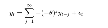
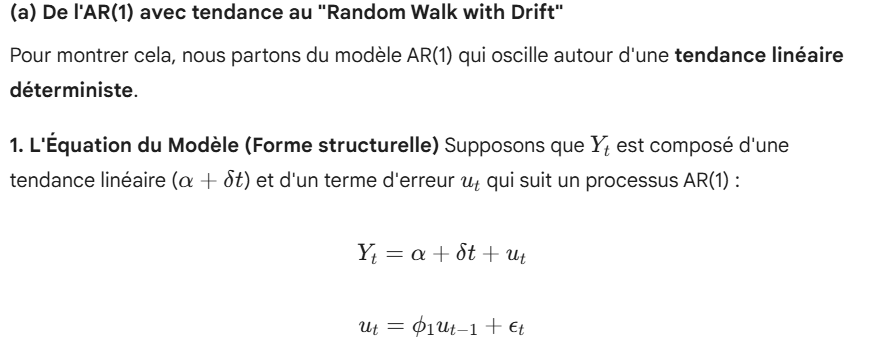
(a) Show that the AR(1) model with deterministic linear

Show that the restricted AR(S) model (where S stands for seasonality) reduces to the seasonal random walk when ϕS = 1.

mu(t ) = mu(t-s) saisonnier

Garch'(1,1) prefered to pure arch(p)

In recent empirical research, GARCH(1,1) models are preferred to pure ARCH(p) models for three main reasons:

1. Parsimony (Efficiency):

   • To properly capture volatility persistence using a pure ARCH model, one often needs a large number of lags (a high $p$), which requires estimating many parameters.

   • A GARCH(1,1) model achieves a similar or better fit with only 3 parameters ($\omega, \alpha, \beta$), making it statistically more efficient and less prone to overfitting.

2. Infinite Memory (ARCH($\infty$) Equivalence):

   • Mathematically, a GARCH(1,1) process is equivalent to an ARCH($\infty$) process.

   • Thanks to the $\beta \sigma_{t-1}^2$ term, the model has "long memory," meaning past shocks decay gradually over time but theoretically never completely disappear. An ARCH(p) model has a finite memory that cuts off abruptly after $p$ lags.

3. Non-Negativity Constraints:

   • Ensuring that the conditional variance remains positive requires all coefficients in an ARCH(p) model to be non-negative. This is difficult to enforce when estimating many parameters. With GARCH(1,1), enforcing positive constraints on just $\alpha$ and $\beta$ is straightforward.

extensions garch

n English (Summary)

1. GARCH-M (in-Mean):

   • Captures: The Risk-Return Trade-off (Risk Premium).

   • It allows the conditional volatility to influence the expected return, testing the theory that higher risk should lead to higher rewards.

2. GJR-GARCH (or EGARCH):

   • Captures: The Leverage Effect (Asymmetry).

   • It accounts for the fact that "bad news" (negative shocks) tends to increase volatility more than "good news" (positive shocks) of the same magnitude.

new impact curve action

1. Symmetric Reaction (Standard GARCH)

In a standard GARCH(1,1) model, the conditional variance depends on the squared past residual ($\epsilon_{t-1}^2$).

• The Shape: The News Impact Curve is a perfectly symmetric parabola (U-shape) centered at zero.

• The Behavior: Because the shock is squared, the sign (+ or -) does not matter.

  • A positive shock (good news, e.g., +5%) and a negative shock (bad news, e.g., -5%) of the same magnitude produce exactly the same increase in future volatility.

• Limitation: It fails to capture the "leverage effect" observed in real markets.

2. Asymmetric Reaction (GJR-GARCH or EGARCH)

These models include a specific term to differentiate between positive and negative shocks.

• The Shape: The curve is asymmetric. It is steeper on the left side (negative shocks) than on the right side (positive shocks).

• The Behavior: The model reacts differently depending on the sign of the shock.

  • Bad news (negative shocks) causes a larger increase in volatility.

  • Good news (positive shocks) causes a smaller increase (or sometimes a decrease) in volatility.

• Key Concept: This successfully captures the Leverage Effect (panic creates more instability than euphoria).

(e) How does conditional heteroscedasticity get detected?

Conditional heteroscedasticity is detected by analyzing the squared residuals ($\epsilon_t^2$) of the model.