STAT115 theory + explanations of equations

Based on practice exam - theory first and then will write out meanings/applications of equations from formula sheet

(prac) Types of Data/Variables

Numerical Variables

• Continuous: take any value in a range (e.g. volume in ml, age)

• Discrete: Take certain numerical values, typically whole numbers (meaningful magnitude, often count) (e.g. number of children in a family, number of cases of cancer diagnosed)

Categorical variables

• Binary/dichotomous: Allocates each case to 1 of 2 categories (e.g. coin lands head or tails (H/T), ind is pet owner or not (yes/no), or represented in numbers 0/1)

• General: Can have 3 or more categories that don’t overlap (e.g. species, blood group A B AB O)

• Nominal: No natural or relevant ordering (e.g. species, blood group)

• Ordinal: Natural order (e.g. degree of pain minimal/moderate/severe)

Note: sometimes ordinal variables analysed as discrete numeric (e.g. indicate level of agreement with a number, 1-5)

Ratios and proportions

Ratio: fraction of one quantity over another (e.g. 10 boys 20 girls, ratio boys to girls 10/20 = ½ = 0.5, ratio girls to boys = 20/10 = 2)

Proportion: Fraction of one quantity compared to the whole (e.g. 10 boys 20 girls, proportion of boys is 10/(10+20) = 1/3, proportion of girls is 20/(10+20) = 2/3)

Converting percentages

To convert proportions to percentages, multiply by 100 and add a % sign.

To convert percentages to proportions, divide by 100 and remove % sign.

e.g. 30% = 0.3, 56% = 0.56

Rates

Ratios for quantities with different units

e.g. Number of road accidents per 1000km travelled

Incidence vs prevalence

Incidence: number of new cases per unit time and population size

Prevalence: existing number of cases at given time per population size

Sample variance

average squared distance between observations and the mean (squared so positive values cancel out the negative values)

If the observations close together, most of the observations minus mean will be small, so variance will be small

Units are squared version of units of original data

Standard deviation

Square root of variance

average deviation of observations from the mean

Approximately 70% of the data will be within one standard deviation of the mean

Approximately 95% of the data will be within two standard deviations of the mean

(prac) Units are the same as the units of the original data

Probability

Set of all possible outcomes is the sample space

must be between 0 and 1, probabilities sum to 1

The probability of an outcome is the proportion of times the outcome occurs if we were to observe the random process a large (infinite) number of times

Probability of mutually exclusive outcomes

(prac) Cannot both happen, in equation Pr(A or B) = Pr(A) + Pr(B) - Pr(A and B), Pr(A and B) is zero

Complement

Complement of event E: the outcomes in the sample space that are not in E

Pr(E) + Pr(E^∁) = 1, or Pr(E) = 1 − Pr(E^∁)

Pr((A and B)^∁)?

• A and B = 1, 3 (in the example)

• A and B complement = 2, 4, 5, 6 = 4/6 = 2/3

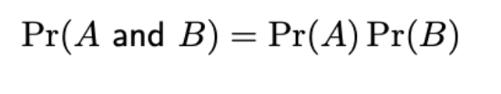
Probability of independent events

Outcome of 1 event does not provide info about outcome of the other

(This isn’t in formula sheet, which I think gives A and B for dependent events)

Conditional probability

probability of event B given event A has occurred is Pr(B | A)

Two events A and B are independent if Pr(B | A) = Pr(B) (event A occurring does not change probability of B occurring)

Contingency table proportions/probabilities

Divide amount of that event by the total

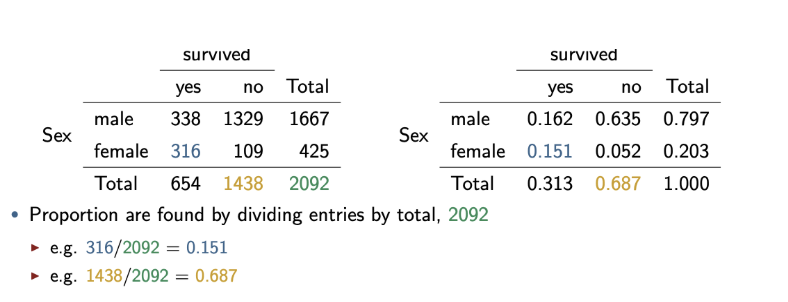
Marginal probability

• e.g. probability male: Pr(M) = 1667/2092 = 0.797

Joint probabilities

• e.g. probability male and survived: Pr(M and S) = 338/2092 = 0.162

Order of joint probability vs conditional probability

Order doesn’t matter for the joint probability

• Pr(A and B) = Pr(B and A)

Order does matter for the conditional probability

• Pr(A | B) and Pr(B | A) are two different quantities

• A given B, or B given A occurred

(prac) Law of total probability (for marginal probability, probability of a single event occurring)

To find Pr(B), sum over possible outcomes that could co-occur with the event B

If there are 2 outcomes: A1, and A2 (which is A1 complement)

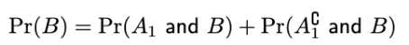
OR if have been given conditional probabilities (like in prac):

Pr(B) = Pr(B|A)*Pr(A) + Pr(B|Ac)*Pr(Ac)

• Ac as in A complement

Tree diagrams

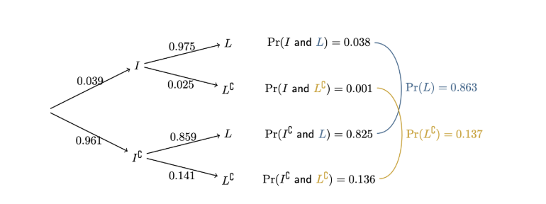
Each set of branches sums to 1 (each event and its complement, e.g. 0.039 + 0.961 = 1)

Times first branch with following branch to get desired probability, e.g. to get Pr(I and L) = 0.039×0.975 = 0.038

Random variables

assigns a numerical value to each outcome in sample space

(prac def): A random variable is a (random) process with a numerical outcome

Represent random variable with capital letter, possible values given with lowercase letters

Discrete vs Continuous random variables

Discrete: distinct values (e.g. number of eggs in a nest)

Continuous: infinite number of possible values — gives probability density:

• Probability given by area under curve, total area under curve is 1

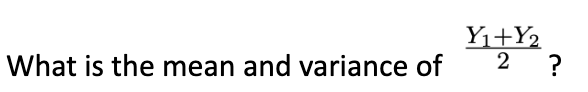
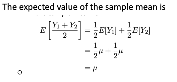
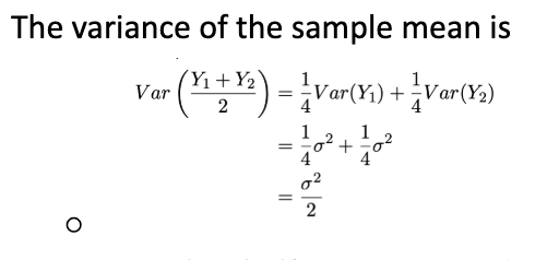
Mean and variance of independent observations from a distribution (of random continuous data)

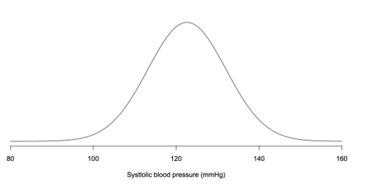
Normal distribution

Bell-shaped curve, Mean µ (peak), Standard deviation σ (or variance σ²)

• µˆ (hat is supposed to be above the µ) = ybar          

  • population mean estimate = sample mean

• σˆ = s           

  • population st dev estimate = sample st dev

Used for continuous random values that have a reasonably symmetric distribution

Values less likely further away from mean

Can transform to remove skew — e.g. log(y) rather than y (using natural base e logarithm)

Z-score

How many standard deviations above (positive z-score) or below (negative z-score) the mean a value is (standardising)

Probability of being within certain z-scores (standard deviations):

•  Pr(−1 < Z < 1) = 0.6827: Approximately 68% of values should be within 1 sd of the mean

• Pr(−2 < Z < 2) = 0.9545: Approximately 95% of values should be within 2 sd of the mean

• Pr(−3 < Z < 3) = 0.9973: More than 99% of values should be within 3 sd of the mean

Probability function for normal distribution (pnorm)

Gives probability a random value is less than a given value (based on z-score, amount of standard variations away from mean)

Find z-score for a value (formula sheet), then do pnorm(z) in R

(prac): pnorm(z) gives probability of a value being less than a given value (z-score of it), 1-pnorm(z) gives probability of a random value being more than a given value (based on z-score of it)

Quantile functions for normal distribution (qnorm)

Find a z-score (q) (amount of standard deviations from mean) for a value that a given percentage are lower than (p)

e.g.

Find the z-value for the time which 1.5% of people’s reaction times are faster (i.e. lower) than. This z-value can be found using qnorm(0.015)

Find the z-value for the time which 1.5% of people’s reaction times are slower (i.e. greater) than. 100-1.5% = 98.5%, use qnorm(0.985) I thinkkkkkk

Sampling distribution

Normal models/distributions have mean µ and standard deviation σ

If take many samples, sample mean (ybar) and sample standard variation will vary from population parameters — Sampling distribution of ybar is how much we expect ybar (sample mean) to vary from one sample to another

Prac: Sample mean will be same as population mean (in theory), sample variance is σ²/n (which means sample standard deviation is squareroot(σ²/n), aka σ/squareroot(n))

estimated with rnorm(n,mean,sd) in R

standard deviation of sampling distribution of ybar also called standard error (estimated with s/squareroot(n)) (so it’s σ-ybar being estimated by s-ybar)

Confidence interval

Prac: for population mean: estimate ± multiplier × standard error (seems to be given in prac exam but just in case)

• uses multiplier (aka critical value) z 1 - alpha/2, with alpha being significance level (= 1 - confidence level as a decimal)

Quantifies how precise estimate of a value (like e.g. the population mean) is, gives upper and lower values that given percentage of sample means will be in (e.g. On average, 95% of sample means will be in this interval, means that confidence interval should contain true mean in 95% of the samples)

For 95% confidence interval, alpha = 0.05, 1-alpha/2 = 0.975, multiplier is z0.975, use qnorm(0.975) to get amount of standard deviations for lower limit idk im confused but this isnt in the prac exam so probably fine

if sample size large enough, confidence intervals reasonable for non-normal data

z-distribution vs t-distribution for normal distributions + confidence intervals for these

Prac: z-distribution (z multiplier) used when population standard deviation is known. t-distribution is used when population standard deviation (σ) has to be estimated (s, sample standard deviation — usually the case as we normally don’t know exact true population parameters)

t-distribution similar to standard normal distribution (z-distribution) but has wider tails. Has additional parameter degrees of freedom (ν > 0), defines how fat tails are

general confidence interval is estimate ± multiplier × standard error, multiplier is z1-alpha/2 (and alpha is 1-confidence level as a decimal)

Prac:

95% confidence interval for population mean using z-distribution: ybar ± z0.975*(σ/sqrt(n))

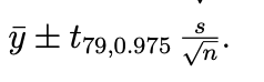
95% confidence interval for population mean using t-distribution: ybar ± tv,1-alpha/2*(s/sqrt(n))

• v = degrees of feedom, which is n-1

• e.g. for sample size 80:

  

(prac) Effect on confidence interval of normal distributions if it is increased

Multiplier (which is either z1-alpha/2 or tv,1-alpha/2, and alpha = 1 - confidence level) changes and interval is wider

E.g. what happens to interval width if we increase confidence level from 95% to 99%

• The interval gets wider (margin of error gets larger)

• Confidence level increases, α decreases (alpha = 1 - conflevel)

• Multiplier increases

Interpreting confidence interval

can find using t.test(dataname,conf.level=whatever) in R

Prac: e.g. for 95% confidence interval, means across many samples, the true value (e.g. population mean) should be in the interval 95% of the time. We are 95% confident that the true value is between the lower and upper limits given.

Wider confidence interval = less precise, quantified by margin of error (half interval width (upper limit - lower limit))

Standard error of normal distributions

Tells us how variable the statistic (e.g. estimate of mean, ybar — or stuff like beta1hat) is across samples/ the sampling distributions (assuming all else held fixed — also larger sample size means ybar more likely to be closer to true mean)

Cannot be negative (like standard deviation, since it measures variability, minimum variability is zero)

using z-distribution to approximate t-distribution

t-distribution or t-multiplier depends on degrees of freedom (v, which is n-1), so if don’t have sample size, can use z-distribution to approximate t-distribution

e.g. If the desired level of accuracy (e.g. 0.04) is given by the symbol ξ, we want to find the value of n such that

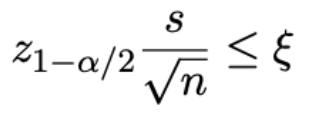
probs don’t need to know all this stuff hopefully, prac exam a lot easier

General hypothesis testing (prac)

Null hypothesis: H0 = claim tested, status quo, or assumption of no difference (e.g. H0: µ = 7 or whatever) 

Alternate hypothesis: HA = other claim being considered, or assumption of difference  (e.g. HA : µ ≠ 7 or whatever)

Hypotheses are about population parameter (so e.g. µ (population mean), not ybar (sample mean))

t.test in R to get p-value etc

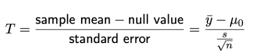
Test statistic for hypothesis testing 

Test statistic used to find how many standard errors separate sample mean from null value (measure how incompatible data is with null hypothesis)

(probs don’t need to know equation since not given in formula sheet)

p-value for general hypothesis testing

Area of lower and upper tail of normal distribution

find with pt(Tstat,df=n-1) in R, times answer by 2 to get p-value (total area of both tails), or just t.test(dataname,mu=nullvalue) to find it

p-value is the probability of observing data as or more extreme than that observed given the null hypothesis is true

Smaller p-value = greater incompatibility between data and null hypothesis (data is unusual if null hypothesis is true, incompatible)

Significance level α=0.05 for 95% confidence level (1-confidencelevel)

If the p-value < α: reject H0

• If the p-value > α: fail to reject H0 (data not unusual if null hypothesis true)

If sample size large enough, p-values reasonable for non-normal data

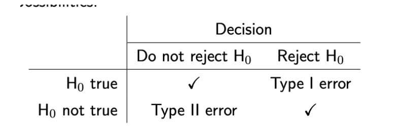
(prac) Type I and Type II errors (+ power)

Type I (α):

Rejecting H0 when it is true

Type I error rate given by alpha, significance level (we get to choose this, 1-confidencelevel)

Decreasing alpha will reduce number of type I errors made (alpha is threshold for incompatibility with null)

Type II (β):

Failing to reject H0 when HA is true (and H0 is not true)

Type II error rate represented as Beta. Power (the probability of rejecting the null hypothesis, given it is incorrect, aka the probability of detecting an effect when there is one) is 1 - beta.

Trade off between type I error rate and power

If we decrease alpha (lower type I error rate), increase type II error rate beta, decrease power.

If we increase alpha (higher type I error rate), decrease type II error rate beta, increase power.

Impact of effect size on power

Effect size is µA − µ0 (difference between values of alternate hypothesis and null hypothesis, amount alternative mean differs from null mean). Larger effect size = more powerful test (all else equal).

Can’t typically control size of effect.

(prac) Impact of sample size on power

Larger sample size = more powerful test (all else equal)

Can control sample size

Effect of population standard deviation on power

Smaller population standard deviation (spread of data around mean) = smaller standard error (estimates the variability of sample means around the true population mean), more precise ybar (sample mean), and more powerful test, all else equal.

Can’t typically control population standard deviation (σ)

what can cause very small p-values, and relationship with confidence intervals

P-value does not measure size of effect or importance of result. if p = 0.0000001 (very small), could be because effect size is large, or could occur when effect size is small (but not zero) and sample size is large.

If testing H0: µ = µ0, HA: µ ≠ µ0, equivalence between p-value and confidence interval: p-value < α is equivalent to µ0 outside the (1 − α)100% confidence interval (e.g. if p-value < 0.05, then µ0 is outside 95% confidence interval — if p-value > 0.01, then µ0 is inside 99% confidence interval)

p-value does not tell us strength of effect, confidence interval gives interval estimate of effect

Comparing 2 means of independent normally distributed data

Group 1 (experimental): normally distributed with mean µ1 and variance σ1^2

Group 2 (control): normally distributed with mean µ2 and variance σ2^2

Difference in means is µ1 − µ2 (or µ2 − µ1): Estimate using ybar1 - ybar2 (or ybar2 - ybar1)

Calculating confidence interval for comparing 2 independent group means (by hand and in R (prac))

By hand:

1. Find sample mean in each group (ybar1, ybar2)

2. Find sample variance in each group (s1², s2²) (seems like we should be given this)

3. Find standard error (formula sheet)

4. Calculate degrees of freedom

5. Find the t-multiplier

6. Construct the confidence interval [Ybar 1 - ybar 2] + or - multiplier * [standard error]

don’t think we’ll need to do the whole process especially as some equations for this aren’t on formula sheet and prac exam isn’t that complicated

(prac) In R:

assign the 2 groups using group1name = subset(dataname, Group == “group1name”), then group2name = subset(dataname, Group == “group2name”) — separate data frames

then use t.test(group1name$data,group2name$data)

Gives confidence interval, also calculates degrees of freedom and group means

(prac) Confidence interval meaning for comparing 2 independent group means

For 95% confidence interval (example):

We are 95% confident that the mean EEG frequency for the control group is between (0.2969, 1.3031) higher than those in solitary confinement

In the long run, we would expect 95% of the confidence intervals we calculate to include the true difference µ1 − µ2 (if we took repeated samples)

prac example:

We are 95% confident that the true difference in mean systolic blood pressure reduction between drug A and drug B (drug A - drug B) is between -1.13 and 7.22.

(calculated using t.test(drugA$reduction, drugB$reduction)

Hypothesis test for comparing 2 independent group means

H0 : µ1 − µ2 = 0 (2 groups have same means)

HA : µ1 − µ2 ≠ 0 (group means differ)

use t.test in R to get p-value

small p-value is evidence in incompatibility between data and null hypothesis, suggests there is a difference between group means (alternate hypothesis)

Paired data hypothesis test

When comparing 2 groups that are not independent

In R: can create difference category (data$difference = data$group1 - data$group2), model as a normal sample — yd (difference between groups) assumed to be normal with mean µd and variance σd^2. µd = mean difference in population.

In R:

can use t.test(data$difference), gives p-value and confidence interval etc.

OR can specify the 2 groups and include paired = TRUE — t.test(data$group1, data$group2, paired = TRUE) (prac)

Interpretation:

confidence interval: We are 95% confident that mean difference in the groups is between (lowerlimit, upperlimit) units

p-value (if smaller than alpha, which is 0.05 for 95% conflevel): evidence data incompatible with null hypothesis (assumption of no difference)

(prac) Correlation (r)

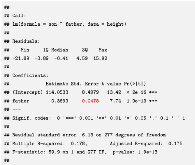
Strength of linear relationship between 2 (continuous) variables (independent variable (x) and dependent variable (y), independent variable influences dependent) — e.g. father’s height vs son height

Between -1 and 1.

Positive correlation: If y is above its mean, then x is likely to be above its mean (and vice versa)

Negative correlation: If y is above its mean, then x is likely to be below its mean (and vice versa)

If the relationship is strong and positive: r will be close to 1

If the relationship is strong and negative: r will be close to −1

If there is no apparent (linear) relationship between x and y: r will be close to 0

In R, use cor(data$independentvariable, data$dependentvariable)

note: r measure linear relationship, strong non-linear relationships can produce r values that do not reflect the strength of the relationship.

Linear regression model

Relationship between continuous variables x (predictor/explanatory/independent variable) and y (outcome/response/dependent variable) — Normal distribution of outcome variable for certain value x (subpopulation)

Probability density for y|x (y given x)

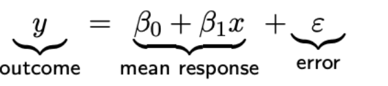
• Intercept β0: where it crosses the y-axis (x = 0) (mean response when x = 0)

• Slope β1

• error = how individual response differs from the mean of their subpopulation (variance of y for value x) — is normally distributed with mean zero and variance σε² — assume it’s zero

observation = mean response + error

Fitted linear regression model

Estimate β0, β1, and y (population parameters) with sample statistics (beta0hat, beta1hat, yhat)

Equation for line of best fit

Residuals

In fitted linear regression model (estimates mean response of y at given x value), observation = fitted model + residual

Residual εˆ (εhat, raw residual) is estimate of error ε, difference between observation (y, actual value) and mean response (yhat, estimate using model)

aka: εˆ = y − βˆ 0 − βˆ 1x

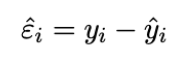
(prac) How are linear regression models fitted?

Want magnitude of the residuals to be as small as possible — use sum of squared residuals, find the values βhat0 and βhat1 that minimise the sum of squared residuals

Found using lm(y ~ x) in R (y is modelled by x)

Interpretation of beta1hat (estimate of slope) and beta0hat (estimate of y-intercept) for fitted linear regression models

For beta1hat: Estimate that y will increase by beta1hat for a 1 unit increase in x.

e.g. We estimate that the average head length of a possum will increase by 0.0573 mm for a 1 mm increase in total length.

For beta0hat: Estimate of y for those with value x = 0 (often doesn’t make sense to interpret)

e.g. βˆ 0 is the estimated mean head length of possums with total length 0 mm

Assumptions for simple linear regression

Linearity: The mean response µy is described by a straight line

Independence: The errors ε1, ε2, . . . , εn are independent

Normality: The error terms ε are normally distributed

 Equal variance: The errors terms all have the same variance, (‘homoscedastic’) σε² (distribution of y around certain value x)

Note: errors are estimated by residuals in practice

How to check linearity (assumptions linear regression)

Visually — fitted line plot, compare observed data to fitted model (line). Underlying data must seem to vaguely follow the line, not be curved, etc.

Can also check for patterns in plot of residuals (raw and studentised) against fitted model line. If there is a pattern, underlying data is not linear.

Studentised/standardised residuals

Difference between observed value (y) and predicted value (yhat) in linear regression model, transformed to have standard deviation around 1. 

Find in R using rstudent(modelname)

How to check independence (assumptions linear regression)

Check that e.g. ε1 tells us nothing about ε2 (errors) (error being the difference between observed value and value estimated by model, estimated by residuals)

Generally difficult to assess, can be checked in data in a time series (close in time = correlated), if data are spatial (close in space = should be correlated), if multiple measurements from each participant (repeated measures, observations from a participant = correlated).

How to check normality (assumptions linear regression)

Errors ε should be normally distributed. Very important for small sample sizes (but hard to check), increasingly less important for large sample sizes (>50), need large violations of normality.

Check for violations using outliers/extreme values:

•  Studentised residuals should be approximately normal with standard deviation 1

  • approx 95% within ±2

  • > 99% within ±3

  • Values exceeding ±4 are unusual: outliers

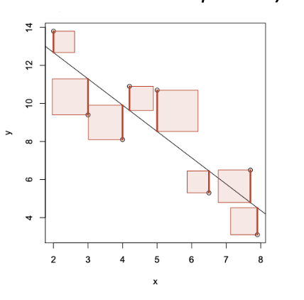
How to check equal variance aka homoscedasticity (assumptions linear regression)

Error terms (ε1, ε2, etc) should have same variance — the magnitude of spread of data around regression line should not change with x.

Violated if data becomes more/less spread around regression line as x changes (along the regression line).

What to do when linear regression assumptions fail

Linearity

• Failure critical, model invalid if data not linear

• Could transform outcome or predictor variables or use different models

Independence or equal variance

• When failed, fitted regression line is usable as value estimate, but confidence intervals and hypothesis tests will be invalid (can’t test uncertainty around line)

• Can be solved using other modelling techniques

Normality/outliers

• Outliers can have dramatic effect on estimated regression

• Check data/outlier values correctly recorded — if they are, consider removing (but think carefully as often outliers interesting, could be revealing something important)

• Be transparent if do remove values

Error variance in linear regression

Error ε (estimated with residuals) assumed to be normal with mean 0 and variance σε²

Larger error variance (all else equal) = larger spread of points around true regression line, more uncertain about fitted regression line (estimates beta0hat and beta1hat less precise)

Esimate of error variance (sε²) = RSS/n-2

RSS = residual sum of squares

(probs won’t need to know equation since not in formula sheet but just in case)

(prac) Standard error of beta1hat

β1 = change in expected value of y for changing x in the population

Estimate betahat1 from observed data — measure precision of estimated slope. using standard error σbetahat1 (standard deviation of sampling distribution of betahat1 = variation is betahat1 across samples)

Standard error proportional to error standard deviation σε

In R (red):

Confidence interval for slope (beta1hat)

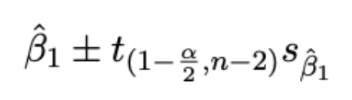
estimate (Beta1hat) ± multiplier (t-distribution with n-2 degrees of freedom (v)) × std error

Outline regression to the mean

E.g. son of short father tends to be short, but on average taller than father. Son of tall father tends to be tall, but on average shorter than father.

Extreme traits regress to the mean.

Hypothesis test for slope (β1) linear regression

Model: y = β0 + β1x + ε (this in formula sheet)

β1 describes how the mean response µy changes with x at population level

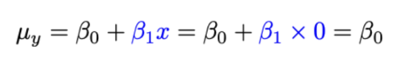
If β1=0 (assume no slope/correlation to hypothesis test this), then y = β0 + ε

• µy = β0: µy does not depend on x (remember we assume error is zero in fitted models)

• Outcome variable is not (linearly) related to the predictor variable

Hypothesis test for β1: H0: β1 = 0 (no relationship between x and y, no slope), HA: β1 ≠ 0 (relationship exists)

To compute p-value (smaller than alpha, 0.05 for 95% conf interval, reject null hypothesis), use t-statistic, t = beta1hat-null/sbeta1hat (standard error of beta1hat)

• And null is zero usually

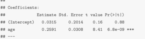
In R (where to find values):

• The test statistic t is given in column t value: 8.41

• The p-value is given in the column Pr(>|t|): 6.8e-09

What is R² (coefficient of determination)

Measure of how well regression model describes data. Squared correlation between y (observed data) and yhat (predicted/fitted data from model). Proportion of variance explained by the model.

In R summary, it’s “Multiple R-squared”

r (correlation) is between -1 and 1, R^2 is between 0 and 1 (0 being model has no use, 1 being model is a perfect fit)

Larger R² = better regression model describes data (fitted/predicted values close to the observations)

Often reported as a percentage

R² = 1-(RSS/TSS) (probably won’t need to know this)

Interpreting R²

No absolute rule of what a good or bad R² value is, can vary based on area of application. High R² value indicates regression model fits data better, but exact desired value varies.

Confidence interval for mean response in linear regression

μyhat = estimate of mean response of y for a given x value

confidence interval = estimate ± multiplier × std error, use t multiplier (since have to estimate standard deviation, with v = n - 2 degrees of freedom).

In R:

Import data using data.frame(dataname = value) — (to construct a data frame), for predictor value (can also find mean response at multiple values using data.frame(dataname = c(value1, value2)

(prac): Use the predict function with option interval = “confidence”

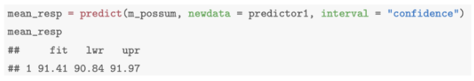
• e.g. We are 95% confident that the mean head length for possums with total length 850 mm is between 90.8 mm and 92 mm

• First argument: model we are using (m possum)

• Second argument (newdata): data frame of predictor values

• Third argument (interval): the kind of interval

• Note: in prac, had to identify the type of interval they were coding for without being able to see whether it was “confidence” based off answer

Rows vs columns in R data frames

Rows: Each row is an observation or data record

Columns: Each column is a variable

Prediction of y in linear regression

use the model to predict a new observation y at a given value of x (prediction of y is same as estimated mean response of y)

Can get from fitted linear regression equation

In R:

use the predict function with option interval = “prediction”

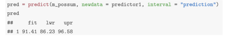
• by default is 95% prediction interval

• e.g. There is a probability of 0.95 that a possum with total length 850 mm will have head length between 86.2 mm and 96.6 mm

• In prac, had to identify whether interval = “confidence” or interval = “prediction” from data output — think prediction interval will have a wider range than the confidence interval?

Multiple linear regression

Have multiple predictors (x1, x2, … , xk, k being number of predictor variables) (predictor variables can be categorical (prac) or numeric, numeric is what we focused on in this course)

y = β0 + β1x1 + · · · + βkxk + ε

• Beta0 = intercept, expected outcome when all predictor variables are 0

• Beta1 … Betak = change in the outcome variable for every 1 unit increase in whatever that x (predictor) value is, all other predictor variables fixed

• remember error is normally distributed with mean 0, so we assume it’s zero when we fit the model

In R, lm(y ~ x1 + x2, data = dataname)

e.g. fitted model:

Note: has same assumptions as simple linear regression

Confidence interval for multiple linear regression

estimate +- multiplier x standard error

multiplier comes from t-distribution, v = n - k - 1

• k being number of predictor variables

• can get estimated standard error from R column Std. error

Use confint(modelname, level=whatever) to get confidence interval

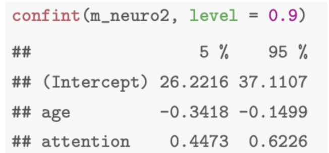
• Prac: Interpreting the confidence interval for β2: We are 90% confident that the average speed score will increase by between 0.4473 and 0.6226 for a one unit increase in the attention score, holding age fixed

Linear regression for categorical predictor variables (2 groups)

2 independent groups, both normally distributed.

Can use dummy or indicator variables to encode the group variables to be numeric — 0 (for control usually) and 1 (for treatment group). Now have quantitative variable and can fit regression model.

So if want to find mean response when x = 0 (group = control):

• β0 is the mean response when x = 0 (when in the control group)

  • β0 = µ1

• β1 is the difference in mean response for x = 1 compared to x = 0 (difference between treatment and control groups, the treatment effect)

  • β1 = µ2 − µ1

In R: make predictor variable (group) a factor variable using as.factor (automatically assigns 0 to group that comes first in the alphabet) then use lm(y ~ x, data = dataname), then summary(modelname)

• e.g. y could be logStool, x could be Group (control (0) or treatment (1))

e.g.

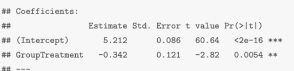
• The estimated expected log(Stool) is β0hat = 5.21 for the control group

• The estimated change in expected log(Stool) with Treatment (compared to Control) is β1hat = −0.34

yhat (aka logStool) = 5.21 - 0.34x (aka Treatment)

Regression models for categorical predictor variables with more than 2 groups

Extend independent group model from previous (where each predictor variable group is normally distributed and independent, and variance is assumed to be the same for all groups)

Use one-way ANOVA (analysis of variance) model — special case of linear regression, divides outcome variables by group. Prac: Compares variance among groups to variance within groups.

(hypothesis stuff was prac): H0 : µ1 = µ2 = . . . = µK

HA : at least one mean is different

In R, use as.factor to make predictor categorical, then use lm(y ~ x, data = dataname) — OR can use aov(modelname) or aov(x ~ y, data = dataname) to get more convenient form

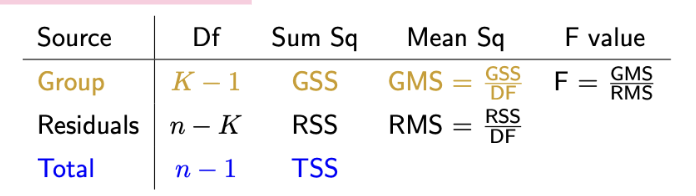
ANOVA table meaning

Prac: The degrees of freedom shown in the ANOVA table are the two values needed to determine the appropriate F-distribution for the test.

Row meanings:

• Group row describes variation between group means (Df, sum sq, mean sq, F value)

• residuals row describes variation within each group, total row describes variation when groups are combined (not in R output)

Column meanings:

• Df = degrees of freedom

• Sum square = sum of groups

• mean square = group (GMS): between-group variance — residual (RMS) estimate of within-group variance

• F value: ratio of group mean square and residual mean square (between-group variance vs within-group variance)

What is the F-value in ANOVA + how can it be used to find a p-value

Compares variance between groups (variability in group means) to variance within groups (measure of how much variation in data is explained by groups). Realisation from an F-distribution if the null hypothesis is true.

If null hypothesis true, all group means will be equal (data will be normally distributed with same mean and variance) and (prac): F-statistic will have F-distribution with Df(group), Df(residual) degrees of freedom.

If null hypothesis true, expect F-value of around 1. If the group means explain a lot of the variation in the data (alternate hypothesis true), the F-value will be large.

An extreme F-value is large, or larger, than that observed — indicative of groups explaining as much or more variation in the data. pvalue is 1-pf(F, df1, df2), so large F-value will result in small p-value (likely to be statistically significant — group explains variation, alternate hypothesis true)

Prac: To determine the p-value, compare F-value to an F-distribution with given df1 and df2 degrees of freedom.

(prac) Issues with pairwise companion of group means (in ANOVA) — multiple comparisons

If compare each group, potentially many comparisons (comparing each group to every other group individually).

Problem with this is that for hypothesis testing, in each test there is a chance of a false positive (type I error, probability of α of rejecting null hypothesis when it is true). With multiple tests, overall chance of type I error increases.

Overall type I error rate = the family-wise error rate, increases with multiple comparisons

What is TukeyHSD

Tukey’s honest significant difference, multiple comparison approach for ANOVA models. Finds corrected confidence intervals and p-values, adjusting for multiple comparisons.

If sample sizes same in each group, family-wise error rate (overall rate) is exactly α. If sample sizes different among groups, error rate is conservative (less than α). 

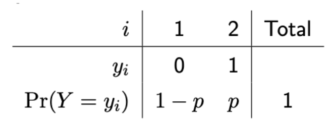
Bernoulli distribution

Discrete probability distribution. Used for binary data (yes/no) — Random variable Y (outcome variable) with 2 possible outcomes, success (represented with 1) or failure (0).

2 outcomes have associated probabilities — represent probability of success with p (aka a proportion)

(prac) What are binomial distributions used for + binomial assumptions

Used when there are many binary trials (Bernoulli trials/distributions, Bernoulli distribution models a single trial). Number of successes from multiple Bernoulli trials has binomial distribution if (binomial assumptions):

• Trials are binary (success/failure)

• Number of trials (n) is fixed (does not depend on number of successes/failures you see)

• Trials are independent

• Probability of success (p) is same for each trial

Number of successes from n independent Bernoulli trials is X = Y1 + Y2 + … Yn

In R: use dbinom(x = numberofsuccesses, size = n (sample size), prob = p (probability of success))

Estimating probability of success (p, binomial distributions) — sample distribution (distribution of sample proportion)

p = parameter (population), estimated with sample statistic phat, number of successes (x) over amount of trials (n)

Sampling distribution for phat is very skewed at high or low probabilities of success for smaller trial (sample) numbers. As sample size gets larger, sampling distribution increasingly normal.

Sampling distribution of phat can be approximated by a normal distribution, provided n is large enough (e.g. np > 10 and n(1 − p) > 10) and p is not too close to 0 or 1 . Use nphat and n(1 − phat) to check if a normal approximation is reasonable

If p close to 0 or 1, takes larger n for sampling distribution to be more normal.

Confidence interval of p (probability of success, distribution of sample proportion, binomial distributions)

Use prop.test(x,n) in R: e.g. We are 95% confident that the probability of myopia (a “success” in this example) in a randomly sampled Australian aged 18-22 is between 0.232 and 0.279

(Prac): Note: confidence intervals require normal distribution to be valid, so sample size must be large enough and proportion far enough from 0 or 1 that distribution of sample proportion is approx normal.

Hypothesis testing of p (probability of success, binomial distributions)

Usually H0: p = p0, HA: p≠p0, p0 being a certain probability of success, defaults to 0.5 in R with prop.test

e.g. If p-value < α = 0.05 there is (strong) evidence that the data are unusual given the null hypothesis is true. The data would be very unusual if the probability of myopia in Australians aged 18-22 was really 0.5 — reject null hypothesis

Central limit theorem + relation to proportions (p)

If have a large sample of independent observations from population with mean µ and standard deviation σ, sampling distribution of Ybar will be approximately normal.

A proportion = a mean, so if n = 5 binary observations,  sample mean is ybar = ⅕*(0 + 0 + 1 + 1 + 0) = 2/5 = 0.4, ybar = phat (sample proportion)

Central limit theorem justifies methodology of confidence intervals and hypothesis tests (even if data not normal) for population mean with one sample (t.test), difference in 2 means (t.test), ANOVA (aov), linear regression (lm), as long as sample size large enough (Generally more than 30).

Compare difference in probabilities/proportions (p, probability of success) + confidence interval and hypothesis test

p1hat-p2hat (estimates)

use z1-α/2 for multiplier for confidence interval (approximate sampling distribution with normal) (if know population standard deviation ig??)

(prac): In R, use prop.test(x,n), x being amount of successes (c(amount1,amount2), n being number of trials (c(samplesize1,samplesize2)

(hypothesis stuff is prac, using prop.test):

H0 : p1 − p2 = 0, aka p1 = p2

HA : p1 − p2 ≠ 0, aka p1 ≠ p2)

If p-value less than alpha (0.05 for 95% confidence interval), data unusual if the 2 groups had a same probability (reject null hypothesis)

Name of 2 alternative ways to compare probabilities (p, probability of success)

Relative Risk and Odds Ratio

Relative Risk (ways to compare probability of 2 groups, p1 and p2)

RR = p1/p2, ratio of probabilities

RR = 1.5 means the risk is 50% higher in group 1 than group 2 (1 means risk is same, below 1 means risk is lower for group 1 than group 2 I think)

Can use to find estimates, confidence intervals, etc

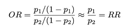
Odds ratio (ways to compare probability of 2 groups, p1 and p2)

If probability of event A is p, then odds of event A are p/(1-p)

Compare 2 groups with an odds ratio: OR = (p1/(1-p1))/(p2/((1-p2))

When p1 and p2 are small:

Tests for independence/association in contingency tables

H0: the 2 variables are independent, HA: the 2 variables are related/associated

If the null hypothesis is true, the test statistic (X² which is on formula sheet never fear) will be a realisation from a χ² (chi squared) distribution with (Rownumber -1) x (Columnnumber -1) degrees of freedom

χ² (chi squared) distribution

Used for tests of independence in contingency tables (prac: H0: the 2 variables are independent, HA: the 2 variables are related/associated). Distribution for positive random variables. Asymmetric (positively skewed), and has 1 parameter (degrees of freedom, (R-1) x (C -1))

p-value given by 1-pchisq(X2, df)

In R: use chisq.test(tablename). If p-value less than alpha, observing a test statistic (X²) as large is unusual if 2 variables independent (reject H0)

χ^2 test is unreliable if any of the expected counts < 5

prac: chisq.test is identical to prop.test in R

(prac) types of research questions

Description: objective of the research is to describe something with no attempt to determine why/the cause.

• e.g. Who is most at risk of injury?

Causation: objective of the research is to evaluate whether or not something (an exposure, treatment) causes a particular outcome in a given population.

• e.g. Does exercise prevent cancer?

Prediction: objective is to determine what we can say about individual units in a population.

• e.g. Is this individual likely to have colon cancer?

Outline the warrior gene case study

Research study in investigate role of a variation of the MAO-A gene in addiction. Reported that proportion of Maori males with low activity allele was higher than more European males. Used to make incorrect comments that Maori carry a warrior gene which makes them more prone to violence, crime, risky behaviour — and thus more involved in things like gambling.

Flaws: study was descriptive, not causation, but treated like it was causation. No discussion with Maori regaring the study. NO data on antisocial behaviour, no evidence for claims. Data from very small non-representative sample. Other issues like previous studies saying MAO-A effect on brain not unique, only linked to antisocial behaviour when maltreated, very varied with ethnicity and genetics.

“Warrior gene” was a term from a monkey study, not relevant to this study, they chose this word to sensationalise the results

Overall failures to consider strength of scientific evidence, place genetic results in context of wider setting, consider the impact of research on Maori, and to communicate well with media.

(prac) CARE Principles (indigenous data)

C: Collective Benefit (for Indigenous people)

A: Authority to Control (by Indigenous people over data)

R: Responsibility (share info about data with Indigenous people)

E: Ethics

Co-design

Type of study design in which researchers, users, participants, and/or communities are involved in every stage of the study (research aims, process, analysis, and outcomes)

Types of sampling (probability sampling)

Population is entire group of interest, sample is subset of the population, sampling frame is list from which sample is drawn (ideally includes whole population). Goal is to get a representative sample.

Simple random sampling:

• Every individual/possible sample has the same probability of being selected.

Stratified sampling:

• Improve representativeness of sample by defining strata (or groups) and taking a simple random sample from each stratum.

• Probability of being selected can be proportional to size of group (useful for understanding overall population), or have an equal number from each stratum (useful for understanding each group and overall population).

• Ensures each group is represented, more precise estimates than simple random sample if parameter varies between groups.

Cluster sampling:

• Single stage: Take simple random sample of clusters (e.g. households, schools, etc — groups in population) and select all units/inds in that cluster.

• 2 stage: Take a simple random sample of clusters, then take a simple random sample of units/inds in each selected cluster.

• Useful when there is no sampling frame of all inds in pop, but is for groups/clusters.

• Often cheaper.

Non-probability sampling

When there is no sampling frame for the pop (required for probability sampling). Members of pop may be difficult to find.

Can be:

• Snowball sampling: sample grown through following contact networks

• Convenience sampling: social media, street corners

• Purposive sampling: selection made using the judgement of a researchers according to the purpose.

2 main sources of error

Estimate from sample can vary from pop truth due to:

• Sampling error: natural random variation between sample statistic and population parameter (magnitude of error captured through confidence intervals and p-values)

• Systematic error (bias): error due to way sample was selected (non-representative), who data obtained from, or quality of data

Often trade-off between random/sampling and systematic error: time/effort spent handling large numbers of respondents vs spending time/effort working on high response rates and quality data (Big Data Paradox)

(prac) Types of biases

Selection bias: when the sample selected is not representative of the population (sampling frame and pop differ)

Non-response bias: those who don’t participate in the study are systematically different from those who do

Information bias: the information provided by respondents is incomplete, or inaccurate

Steps of critical appraisal of studies

1. Summarise study

2. Internal validity (what do findings tell us about population studied — sources of bias, confounding, impact of random variation)

3. External validity/generalisability (what do findings tell us about other populations)

Prevalence vs incidence (of disease)

Prevalence rate: number of existing cases at a given time per population size (e.g. 2 people out of 10 have it at a fixed point in time, 2/10 = 0.2)

Incidence rate: number of new cases of disease per unit time and population size (requires follow-up with people initially free from disease)

• Cumulative incidence = measure of risk, probability an ind develops disease over fixed time period (will be biased estimate of true risk if some people withdraw from follow-up and outcome unknown)

• e.g. 7 people didn’t have disease, 4 developed it during the time period, incidence rate = 4/7

Ways to compare disease frequency

Differences

• in risk (cumulative incidence)

• in incidence rates

Ratios (generally used for studying causation)

• of probabilities

  • prevalence ratio

  • risk ratio (ratio of cumulative incidences, aka relative risk)

• Rate ratio — of incidence rates

• Odds ratio — of odds (often used where there is a binary outcome, can approximate risk ratio for rare outcomes)

• Hazard ratio — interpreted as risk ratios, used where data are a time until an event (e.g. disease) occurs

Individual casual effects

Can never observe 2 diff scenarios of an ind (e.g. taking a pill or not taking a pill), so can never estimate individual causal effect

Estimating casual effects

Average Causal Effect of A versus B compares expected outcome in a pop with treatment A to expected outcome in same pop with treatment B (all else the same) — not individual casual effects

Can estimate by comparing what happens with an exposure/intervention/treatment group to control group (absence of exposure/intervention) — an experiment (randomisation is a critical tool)