Chapter 5 - Investigating and Modelling Time Series

Investigating and Modelling Time Series in a flashcard.

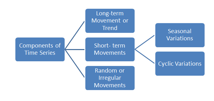
Key Components of Time Series Analysis

1. Time as the Explanatory Variable: Plotted in time order, connected by line segments.

2. Trend: Long-term direction (increasing, decreasing, stable).

3. Cycles: Repetitive fluctuations more than one year.

4. Seasonality: Regular, calendar-related fluctuations (peaks/troughs at consistent intervals).

5. Structural Change: Abrupt, sustained change over 6 months or more.

6. Outliers: Unusually large or small values due to one-off events.

7. Irregular Fluctuations: Short-term, random fluctuations unrelated to trends or seasons.

Time Series Construction

• Horizontal Scale: Label time intervals clearly.

• Vertical Axis: Label with appropriate scale for the response variable.

• Plot Points: Connect points with straight line segments.

• Key (if necessary): Define variables or labels.

• Trend, Seasonality, Cycles: Analyze components based on the graph.

Identifying Seasonality and Cycles

• Seasonality: Regular, calendar-related fluctuations (e.g., yearly). Identified by consistent peaks/troughs with the same magnitude and frequency.

• Cycles: Recurrent movements over time periods longer than one year. Identified by irregular frequency and magnitude.

Structural Change and Outliers

• Structural Change: An abrupt, sustained shift in the level of the series (6+ months or 3+ quarters).

• Outliers: Unusually large or small values, often due to real-world events, distorting trends and seasonality.

Irregular Fluctuations in Time Series

Irregular fluctuations are short-term, unpredictable fluctuations that do not follow any patterns, and they can mask underlying trends and seasonality.

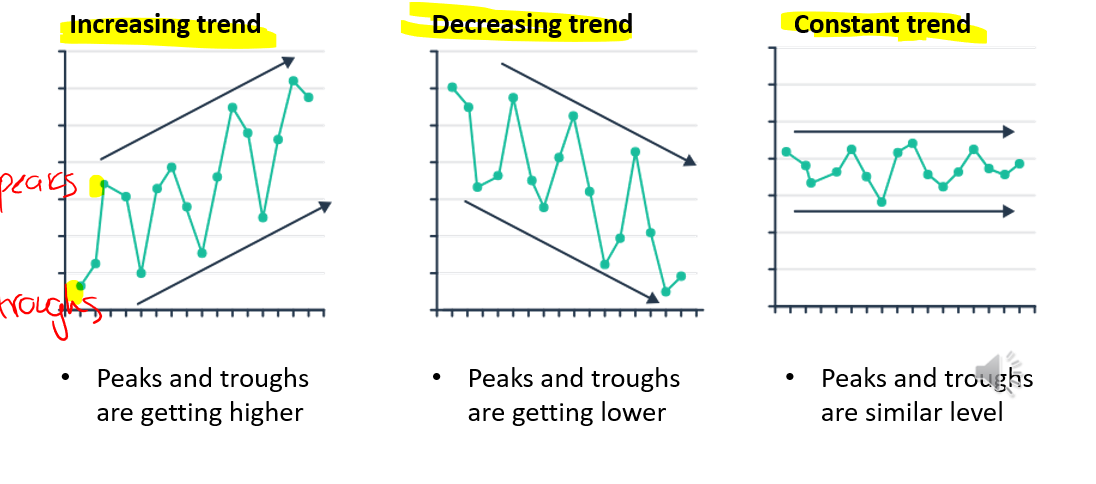
Trend

The 'long term' movement in a time series without calendar related and irregular effects and reflects the underlying level.

By looking at the graph we can see overall whether the response variable is increasing, decreasing, or stable.

Note: DO NOT saying positive or negative trend or positively or negatively skewed

Purpose of Smoothing

Smoothing removes large fluctuations, reducing peaks and troughs to emphasize trends in the data. It helps in investigating the underlying pattern by replacing original data values with calculated means.

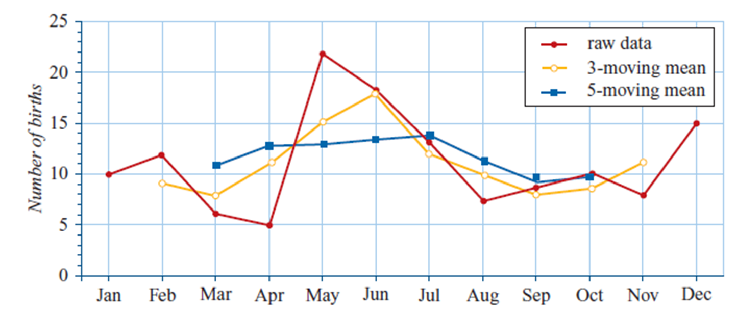
The greater the number of points smoothed, the stronger the smoothing effect, but it also results in more data being lost.

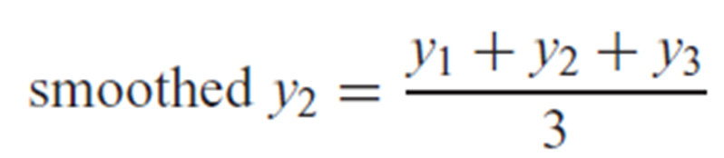
Smoothing Process 1 (3-Point Moving Mean)

Replace each response variable data value with the mean of the value and its two neighbouring values (one on each side). The first and last points are omitted because they cannot be smoothed.

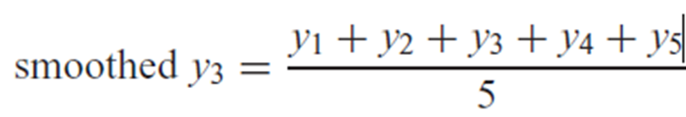
Smoothing Process 2 (5-Point Moving Mean)

Replace each response variable data value with the mean of the value and its four neighbouring values (two on each side). The first, second, and second last, last points are omitted because they cannot be smoothed.

Smoothing with Even Number Points and Centring

Using an even number of points causes the means not to line up correctly with the time period. This issue is resolved by applying 'centring' to shift the mean to the appropriate time period.

Two and Four Mean Smoothing with Centring

• Write down 5 values centred around the required value.

• Calculate the mean of the first 4 values (mean 1) and the last 4 values (mean 2).

• Find the mean of the two calculated means.

• Place the final mean at the centre of the two means.

Odd Number Mean Smoothing

• Find the numbers to be used around the desired value.

• Calculate the mean of these values.

• Place the mean in the middle of the group and repeat for all data points.

Even Number Mean Smoothing with Centring

• Find numbers around the desired value.

• Calculate the mean of the first and second group of numbers.

• Calculate the mean of these two means.

• Centre the final mean and repeat for all data points.

CAS: How to smooth data

Use TimeSII Program and proceed.

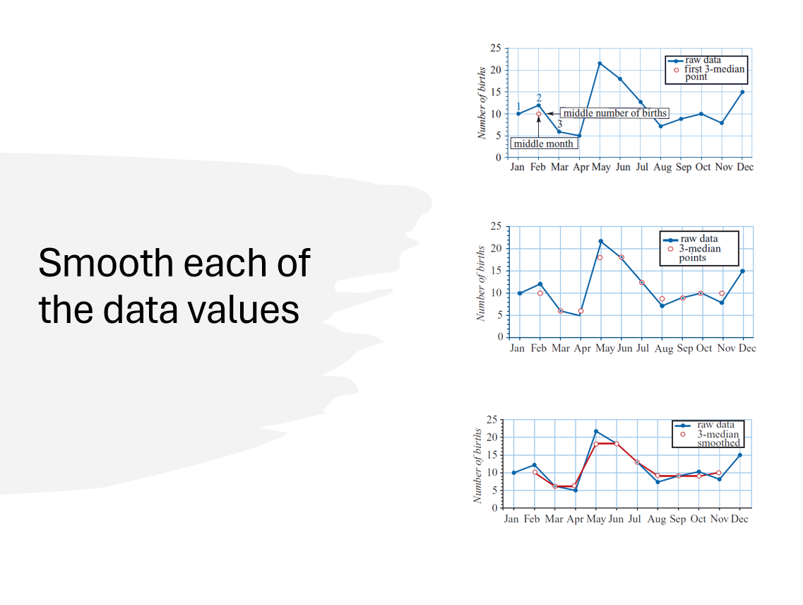
Purpose of Moving Median Smoothing + How to apply

It smooths trends by removing irregular fluctuations, variations, or outliers without needing the actual values and is not influenced by single outliers.

Replace each data value with the median of that value and its two neighbours. This process removes one point from either side of the time series.

For each data point, replace it with the median of the value and its two neighbours. For larger windows (e.g., 5 points), calculate the median of 5 points and place it at the center of the window.

Smoothing in 2D (Graphical Approach)

Identify the horizontal and vertical middle values, find the intersection, and use it as the smoothed median. Repeat for each data point and connect the results.

Seasonal Indices Overview

A seasonal index is a multiplier that indicates how a season’s value compares to the yearly average. It is calculated by dividing the seasonal value by the seasonal (or yearly) average. It shows the percentage increase or decrease from the average.

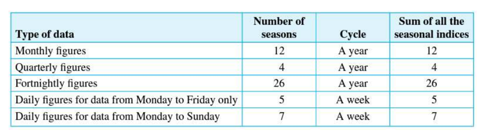
The average of all indices equals 1. Sum of the seasonal indices equals the number of seasons.

Seasonal Index Interpretation

Seasonal indices	< 1	= 1	> 1
Seasonal Indices e.g.	0.85	1	1.23
Describing the seasonal average	15% below	Matches	23% above

A seasonal index >1 means above average, and <1 means below average.

Positive value, then the season is above average by value %;

Negative value, then the season is below average by value %.

Deseasonalising Data

Deseasonalised Figure = Actual Figure / Seasonal Index.

This removes the seasonal component from the data to better reveal trends.

General Equation for Calculating Seasonal Index/Average

𝑠𝑒𝑎𝑠𝑜𝑛𝑎𝑙 𝑖𝑛𝑑𝑒𝑥 = (𝑣𝑎𝑙𝑢𝑒 𝑓𝑜𝑟 𝑠𝑒𝑎𝑠𝑜𝑛)/(𝑠𝑒𝑎𝑠𝑜𝑛𝑎𝑙 𝑎𝑣𝑒𝑟𝑎𝑔𝑒)

Note: Seasonal average can also be called yearly average.

𝑠𝑒𝑎𝑠𝑜𝑛𝑎𝑙 𝑎𝑣𝑒𝑟𝑎𝑔𝑒 = (𝑠𝑢𝑚 𝑜𝑓 𝑠𝑒𝑎𝑠𝑜𝑛 𝑣𝑎𝑙𝑢𝑒𝑠)/(𝑁𝑢𝑚𝑏𝑒𝑟 𝑜𝑓 𝑠𝑒𝑎𝑠𝑜𝑛𝑠 𝑝𝑒𝑟 𝑦𝑒𝑎𝑟)

Re-seasonalising Data

Re-seasonalised Figure = Deseasonalised Figure × Seasonal Index.

This process reintroduces the seasonal component to the adjusted data.

Sample Interpretation: Seasonal Index

The seasonal index for [State EV] (state the seasonal indices) tells us that the figure for [State EV] is (State %) [higher/lower/matches] than the [State number of seasons] average.

Note that the number of seasons can be:

• Yearly

• Quarterly

• Monthly

• Weekly

• Fortnightly

• Daily

Purpose of Smoothing Time Series Data

The purpose of smoothing time series data is to remove peaks and troughs, allowing the underlying trend to be clearer. Once smoothed, if the data appears linear, a least-squares regression line can be fitted. This regression line helps identify trends and is used for forecasting future values.

Fitting Trendlines to Time Series

To fit a trendline, use time as the explanatory variable and apply a least-squares regression. Data may be smoothed or de-seasonalised before fitting the line. The regression line helps identify the trend (positive, negative, or constant) in the data.
General Equation:
Response Variable = a + b × time
This line can then be used for forecasting future values.

Forecasting

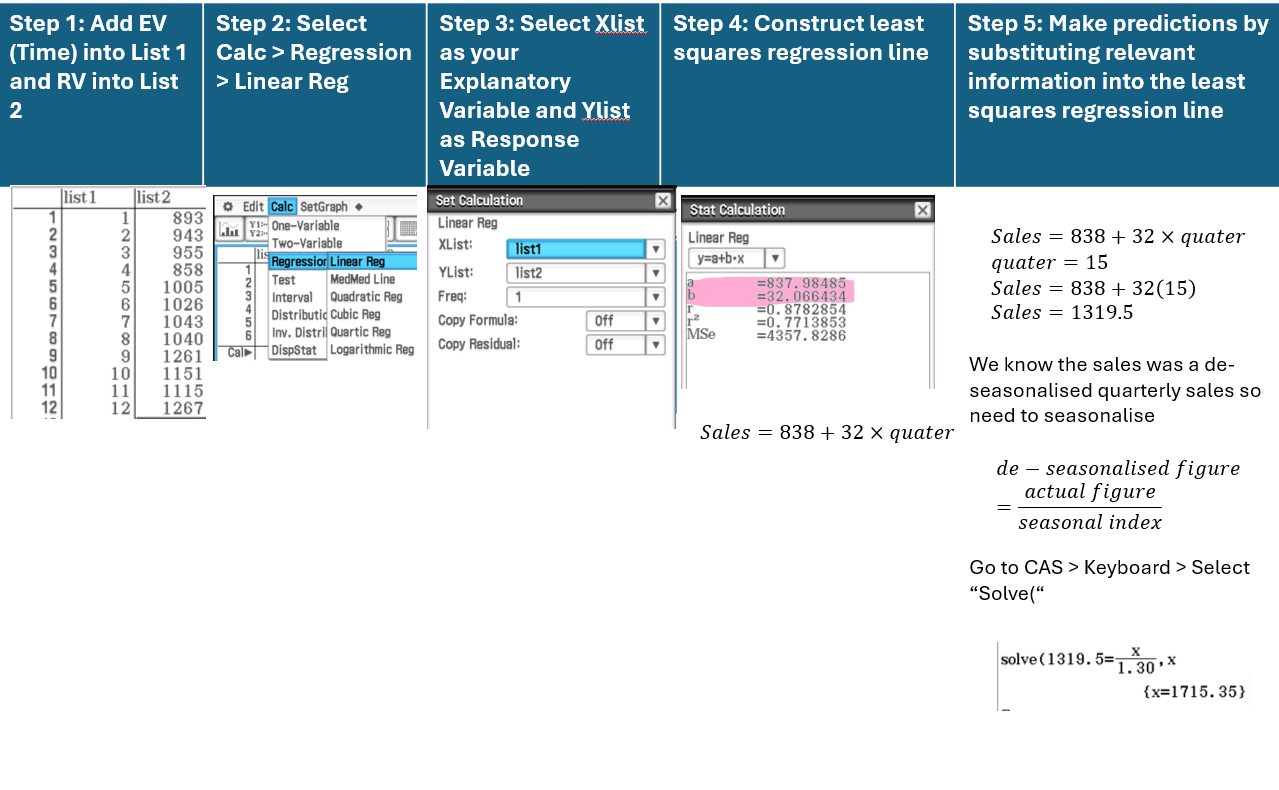
Forecasting = a + b × time
If the data was de-seasonalised, re-seasonalise the prediction using:
Seasonal Prediction = de-seasonalised figure × seasonal index
Where:

• a is the predicted starting value of the time series.

• b represents the rate of trend increase or decrease.
  Ensure the correct seasonal index is applied for re-seasonalisation.

Keep in mind…

• Step 1: Use moving average or de-seasonalised data to find the regression line.

• Step 2: If data is de-seasonalised, re-seasonalise the prediction using:
  Seasonal Prediction = de-seasonalised figure × seasonal index
  Where the de-seasonalised figure comes from the trend line or is given.

• Note: Correlation is not typically relevant in time series since the smoothed line usually has strong, linear correlation.

• Important: Predictions are considered within one cycle of the data and are future predictions, not interpolation or extrapolation.

• Step 3: Always show working:

  • State the value of t (time).

  • Provide the equation of the regression line.

  • Use the correct seasonal index for re-seasonalising.

Template to use when interpreting forcasting

The slope of the regression line predicts that, on average, the [State Response Variable] increases/decreases by [State b].

Fitting Trend Lines with De-Seasonalised Data

• Step 1: Fit the de-seasonalised data to a trend line using linear regression.

• Step 2: Obtain the equation of the regression line:
  Response Variable = a + b × time

• Step 3: Use the equation to predict future values based on time.

• Step 4: Depending on the question, either:

  • Find the de-seasonalised value from the trend line.

  • Or re-seasonalise to find the actual data value using:
    Seasonal Prediction = de-seasonalised figure × seasonal index

(Sometimes, we may be using de-seasonalised data when fitting trend lines)

CAS Instruction: Forecasting