Preferences, Utility, and Optimal Choice

what are the axioms of rational choice

• completeness: if A and B are any two situations, an individual can always specify exactly one of these possibilities unless they have bounded rationality:

  • A is preferred to B

  • B is preferred to A 

  • A and B are equally attractive

• transitivity: if A is preferred to B, and B is preferred to C, then A is preferred to C 

  • individual choices are internally consistent 

  • unless paradox of voting where there are 3 options and 3 voers

• continuity: if A is preferred to B, then situations close to A must also be preferred to B 

  • used to analyse individuals’ responses to relatively small changes in income and prices 

  • unless perfect complements 

describe utility rankings

• assuming completeness, transitivity, and continuity people can rank all possible situations from the least desirable to the most

• if A is preferred to B then the utility assigned to A exceeds the utility of B

  • U(A) > U(B)

• utility rankings are ordinal in nature (no specific values assigned)

  • utility is not necessarily cardinal: to derive demand curves do not need to consider how much more utility is gained from A than B 

  • preferences can be represented by any monotonic transformation of the utility function 

  • for choice under certainty may need cardinality (numerical value assigned)

what is not required for consumer theory under certainty

inter-personal comparability

arguments of utility functions

• utility from consumption of goods

  • if an individual must choose among consumption goods x₁, x₂, … x_n

  • her rankings are given by the utility = U(x₁, x₂,…x_n)

describe well behaved preferences 

may impose more structure on preference by assuming monotonicity and convexity 

• monotonicity (non-satiation): more is preferred to less 

• convexity: we prefer averages to extremes 

describe the characteristics of indifference curves

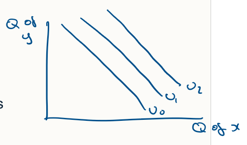
• IC shows the set of consumption bundles about which the individual is indifferent. all the bundles provide the same level of utility.

• negatively sloping due to monotonicity

• convex to the origin due to convexity

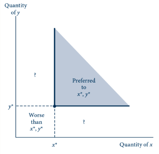
describe the indifference curve for monotonicity

• shaded area: combination of x and y unambiguously preferred to the combination x^*, y^*

• combinations identified by ? ambiguous since they contain more of one good and less of the other

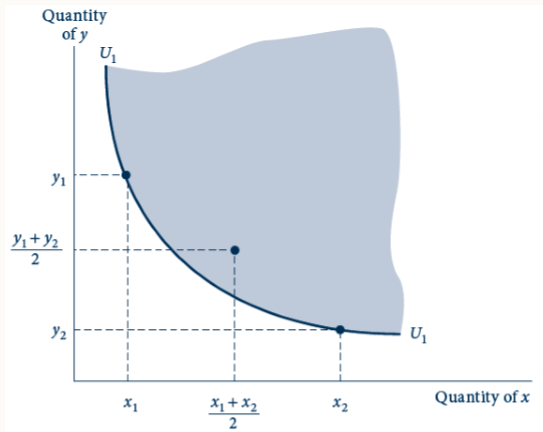
describe convexity 

if indifference curves are convex, they obey diminishing MRS, then the line joining any two points that are indifferent will contain points preferred to either of the initial combinations. balanced bundles are preferred to unbalanced ones. 

• The curve U1 represents the combinations of x and y from which the individual derives the same utility. The slope of the curve represents the rate at which the individual is willing to trade x for y while remaining equally well of. The slope is termed the marginal rate of substitution. Slope has a diminishing MRS

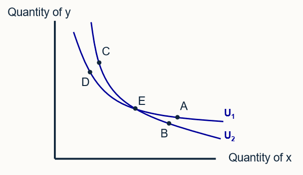
describe how transitivity means ICs can’t cross

• D and A indifferent since on same IC

• but by transitivity, A>B, B and C indifferent, and C>D, so A>D

• By the assumption of nonsatiation (more of a good always increases utility), “A is preferred to B” and “C is preferred to D”. But this person is equally satisfied with B and C as they lie on the same indifference curve, so the axiom of transitivity implies that A must be preferred to D. But that cannot be true because A and D lie on the same indifference curve and are by definition equally desirable. Hence indifference curves cannot intersect.

• E cannot represent two different levels of utility

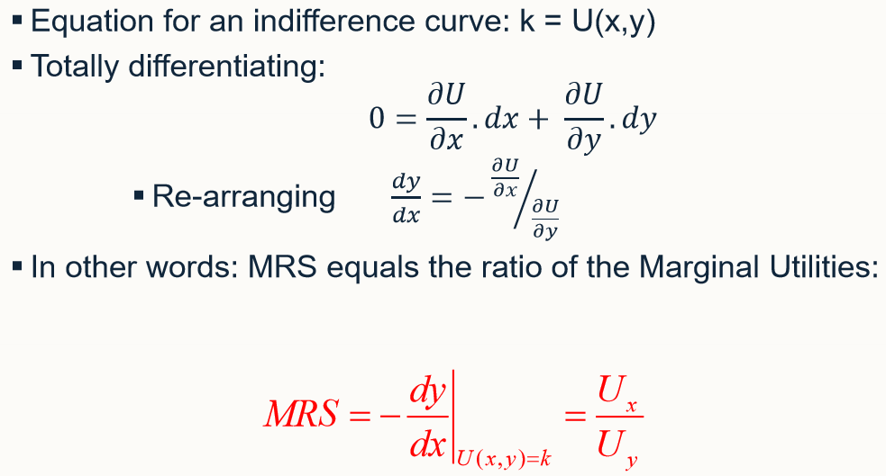
definition of MRS and equation

• the negative of the slope of an indifference curve at some point

• MRS = -dy/dx

• MRS reflects the individual’s willingness to trade y for x

• MRS is how many units of y would be needed to compensate for the loss of 1 unit of x

• convexity of IC reflects diminishing MRS: MRS falls as x rises

  • x becomes less valuable at the margin: you would accept smaller amounts of y in exchange for x

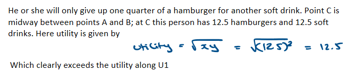
find the MRS for sqrt(xy) if utility is 10. x is soft drinks and y is hamburgers

• MRS = 100/x² 

  • as x rises, MRS falls

complete the mathematical derivation of the IC MRS

• The rate at which x can be traded for y is given by the negative of the ratio of the marginal utility of good x to that of good y. Assuming additional amounts of both goods provide added utility, this trade off rate will be negative, implying that increases in the quantity of good x must be met by decreases in the quantity of good y to keep utility constant.

• MRS at a particular combination of goods will be unchanged no matter what specific utility ranking is used.

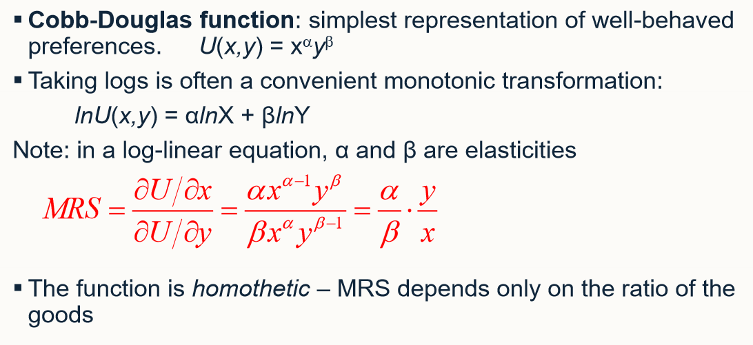
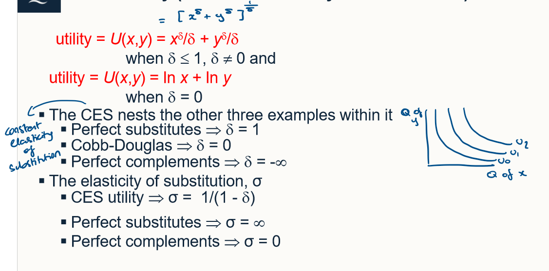
find the MRS of a cobb-douglas functions 

• MRS is homethetic - MRS only depends on the ratio of the goods 

describe perfect substitutes MRS

• linear indifference curves

• utility = U(x,y) = alpha x + beta Y

• MRS = alpha / beta

• MRS is constant along the indifference curves

• A person with these preferences would be willing to give up the same amount of y to get one more x no matter how much x was being consumed

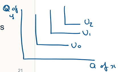
describe perfect complements MRS

• L shaped indifference curves

• utility = U(x,y) = min (alpha x, beta y)

• can’t differentiate this function, an example of discontinuous preferences

• MRS is infinity if y/x > alpha/beta

• MRS = 0 if y/x < alpha/beta

• MRS is undefined if y/x = alpha/beta

• by only choosing goods together can utility be increased

describe constant elasticity of substitution 

describe rationality in economics

• a consumer is rational if she picks the consumption bundle that maximises her utility

  • acted according to the axioms of choice, especially transitivity (she is consistent)

  • does not necessarily mean she is selfish, depends on the arguments of her utility function

  • does not necessarily mean she explicitly calculates the optimal solutions.

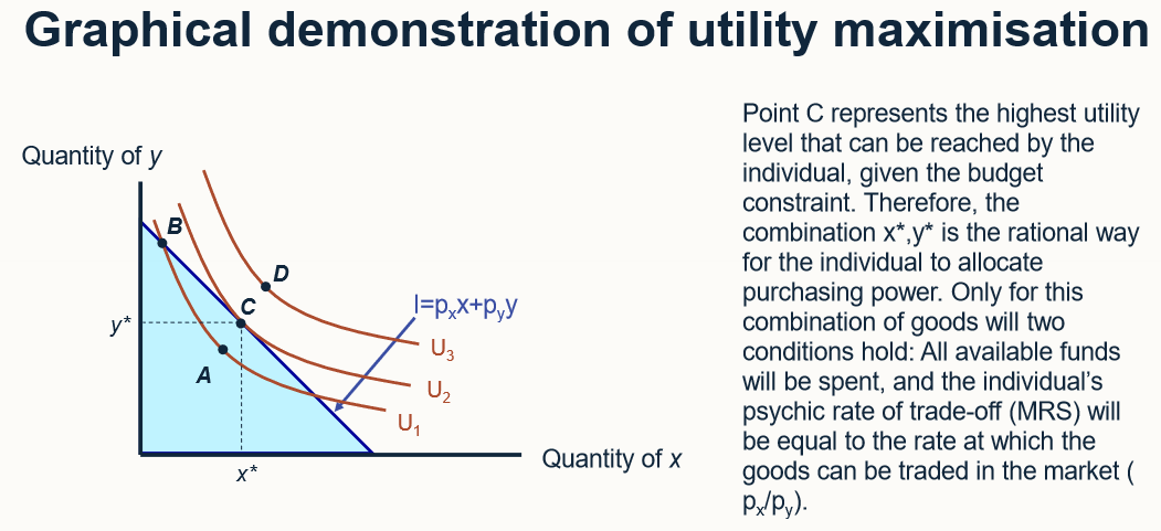
  • Utility maximization. To maximize utility, given a fixed amount of income to spend, an individual will buy those quantities of goods that exhaust his or her total income and for which the psychical rate of trade-off between any two goods (the MRS) is equal to the rate at which the goods can be traded one for the other in the marketplace.

how to calculate optimal choice steps 

• write down utility maximising condition, subject to budget constraint 

• set up the lagrangian

• do FOC 

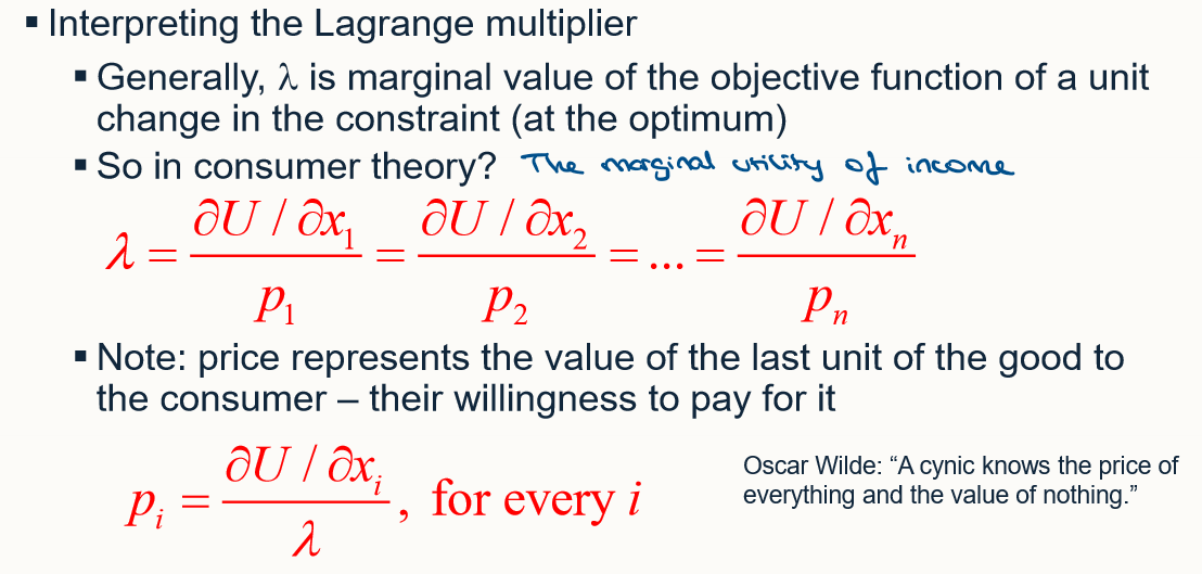
• MRS = (dU/dX_i) / (dU/dX_j) = p_i / p_j

• slope of budget constraint = slope of IC  

  • p_x / p_y = - dy/dx = MRS of x for y

draw a graphical demonstration of utility maximisation

• The individual would be irrational to choose A as they can get to a higher utility level just by spending more of their income. The assumption of non satiation implies that a person should spend all of his or her income to receive maximum utility. By reallocating expenditures, the individual can do better than B. D is out of the question because income is not large enough to purchase D. It is clear the position of maximum utility is C where x* and y* is chosen.

what is lambda in the lagrange multipler?

lambda is the marginal value of the objective function of a unit change in the constraint at the optimum

• At the utility maximising point, each good purchased should yield the same marginal utility per dollar spent on that good. Therefore, each good should have an identical (marginal) benefit to marginal cost ratio. If this were not true, one good would promise more marginal enjoyment per dollar than some other good, and funds would not be optimally allocated.

• The Lagrange multiplier represents the marginal utility of an extra dollar of income, no matter where it is spent. Therefore, compares the extra utility of one more unit of I to this common value of a marginal dollar in spending.

• To be purchased, the utility value of an extra unit of a good must be worth, in dollar terms, the price the person must pay for it. For example, a high price for good i can only be justified if it also provides a great deal of extra utility. At the margin, therefore, the price of a good reflects an individual’s willingness to pay for one more unit. This is a result of considerable importance in applied welfare economic because willingness to pay can be inferred from market reactions to prices.

describe SOC

• differentiate FOC again and check if negative

• if there is diminishing marginal utility, the SOC will hold

• if the MRS is diminishing, the tangency condition will be the maximum

  • for the Cobb-Douglas function, MRS is diminishing so the FOC gives the maximum

  • utility functions that are monotonic and quasi-concave (convex IC) have diminishing MRS

describe corner solutions

• for corner solutions, at the optimal point, the budget constraint is flatter than the IC 

  • rate at which x can be traded for y is lower than the MRS so we just consume x

• Hence the optimal conditions are as before, except that any good whose price p1 exceeds its marginal value to the consumer will not be purchased xi = 0. Thus, the mathematical results conform to the commonsense idea that individuals will not purchase goods that they believe are not worth the money.

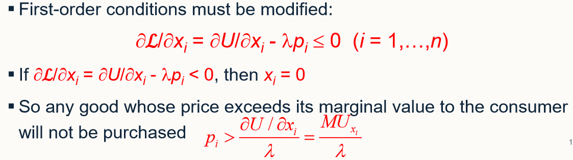
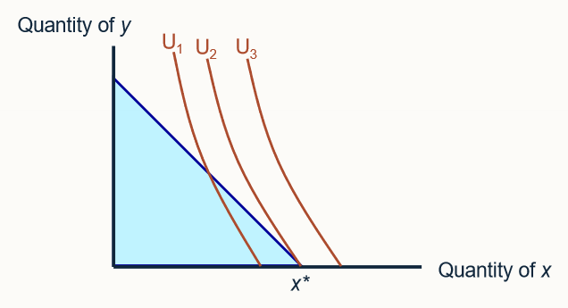
describe this corner solution

with the preferences represented by this set of indifference curves, utility maximisation occurs at x^*, where 0 amounts of good y are consumed. the slope of the ICs are steeper than the BL: we value x more than we can exchange y for it, so we just consume x 

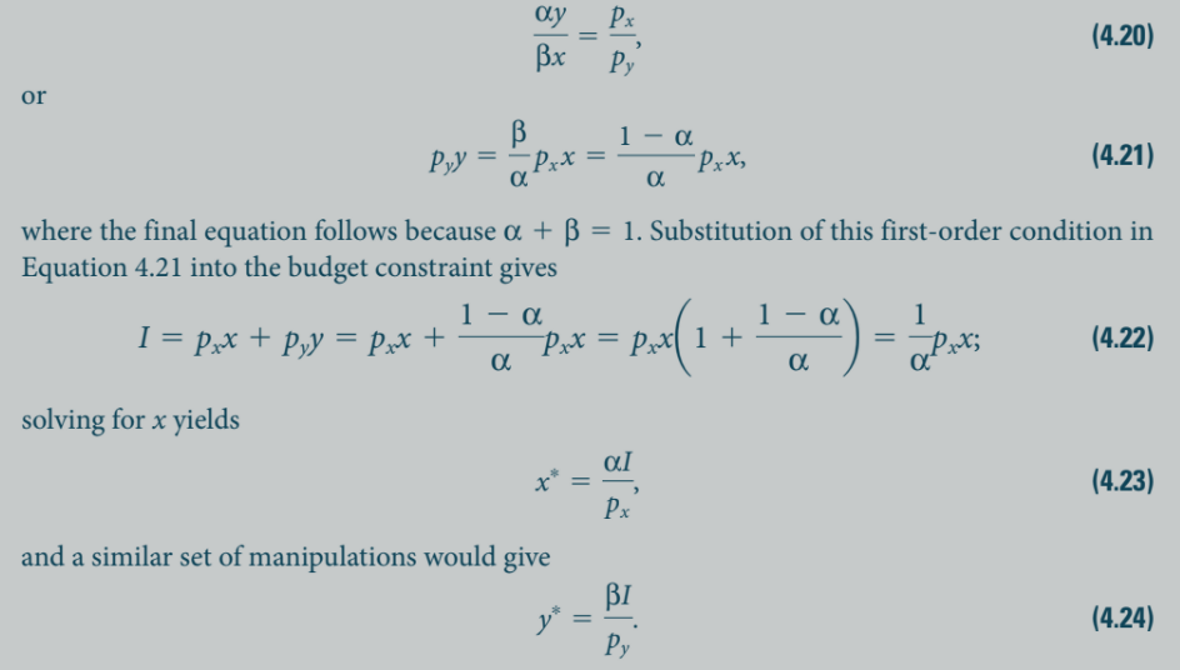
set up the utility function, lagrangian and FOC for the cobb douglas function

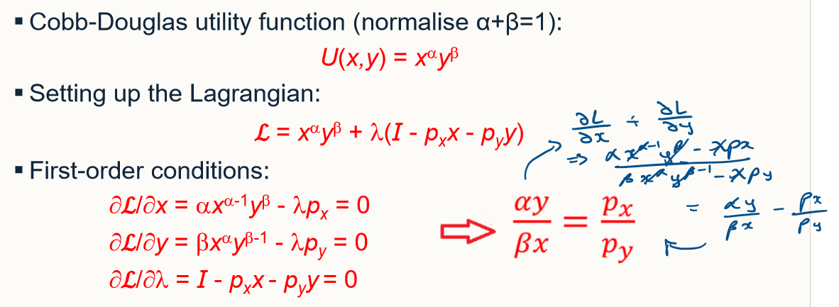
derive the demand function for cobb douglas

hence x^* = alpha I/p_x and y^* = beta I/p_y

• the individual will allocate fraction alpha of his income to good x and fraction beta of his income to good y

• these budget shares are constant and demand depends only on income and own price

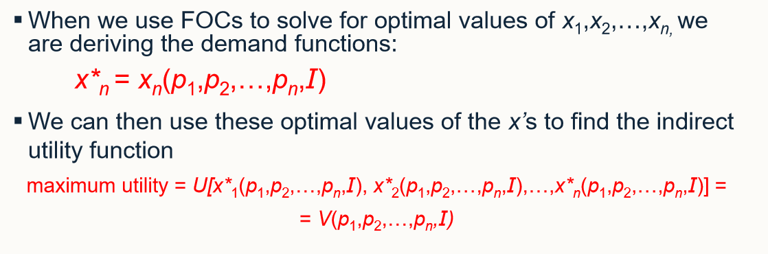
how to find the indirect utility function

v(p1, p2,…pn,I)

the optimal level of utility will depend indirectly on prices and income.

• In words, because of the individual’s desire to maximize utility given a budget constraint, the optimal level of utility obtainable will depend indirectly on the prices of the goods being bought and the individual’s income. This dependence is reflected by the indirect utility function V. If either prices or income were to change, the level of utility that could be attained would also be affected.

find the indirect utility function with cobb douglas U(x,y) = x^alphay^beta. suppose alpha = beta = 0.5

• recall in the generic case, x* = alpha I/p_x and y* = beta I/p_y

• hence we know that x* = I/2p_x and y* = I/2p_y

• so the indirect utility function is:

  • V(p_x, p_y, I) = (x*)^0.5(y*)^0.5 = I / 2p_x^0.5p_y^0.5

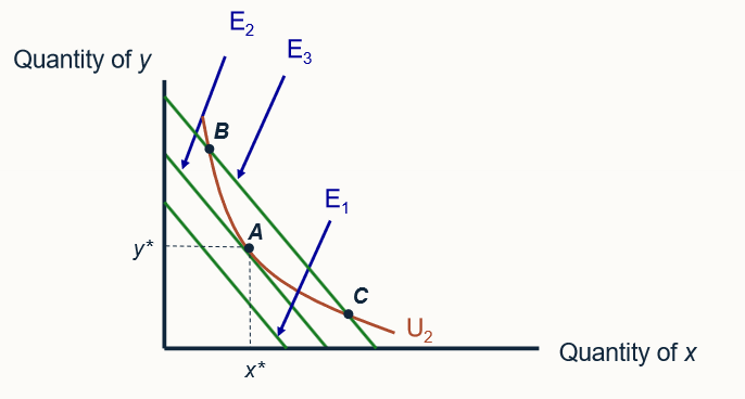
describe expenditure minimisation

the dual of the utility-maximisation problem is to attain a given utility level (U2) with minimal expenditures. an expenditure level of E1 does not permit U2 to be reached, whereas E3 provides more spending power than is strictly necessary. with expenditure E2, this person can just reach U2 by consuming x* and y*

• There, the individual must attain utility level U2; this is now the constraint in the problem. Three possible expenditure amounts (E1, E2, and E3) are shown as three “budget constraint” lines in the figure. Expenditure level E1 is clearly too small to achieve U2; hence it cannot solve the dual problem. With expenditures given by E3, the individual can reach U2 (at either of the two points B or C), but this is not the minimal expenditure level required. Rather, E2 clearly provides just enough total expenditures to reach U2 (at point A), and this is in fact the solution to the dual problem.

describe the dual approach to optimal choice

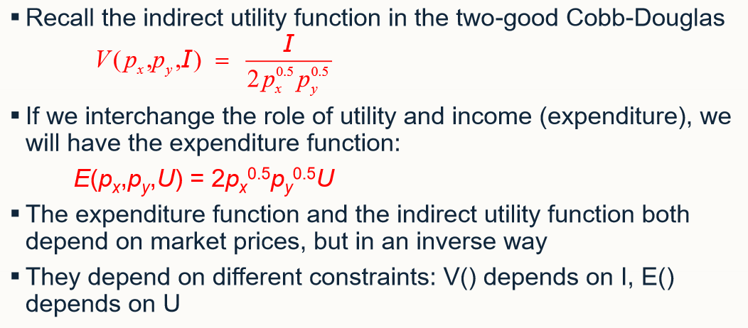
what is the expenditure function for cobb-douglas utility?

• if we interchange the role of utility and income (expenditure), we have the expenditure function

• the expenditure function and the indirect utility function both depend on market prices, but in an inverse way.

• they depend on different constraints: V depends on I, E depends on U

what are well-behaved preferences

an interior solution where the cosumer’’s valuation of the last unit (MRS) is just equal to the rate at which it can be exchanged (relative prices)