Lecture 1

Summary

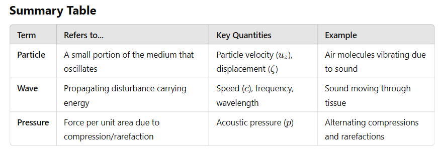
Chapter 1: Introduction to Medical ImagingWhat is Medical Imaging?

- Seeks to view internal structures non-invasively, unlike looking or endoscopy which only shows surfaces.

- True medical imaging gives 3D spatially resolved information.

Applications and Device Selection

- Different imaging techniques used depending on:

- Clinical task

- Safety

- Cost

- Patient-friendliness

- Trade-offs: e.g., ultrasound is cheap and safe but noisy; MRI is detailed but costly.

Categories of Medical Imaging Signals

- Transmission (e.g., X-rays)

- Reflection (e.g., ultrasound)

- Emission (e.g., PET)

- Resonance (e.g., MRI)

Noise in Imaging

- Defined as unwanted signal (e.g., thermal, motion noise).

- White noise model:

y = s + e, \quad e \sim \mathcal{N}(0, \sigma^2)

- SNR improves with averaging: \text{SNR} \propto \sqrt{N}

Contrast and CNR

- Contrast:

C_{AB} = |S_A - S_B|

- Contrast-to-Noise Ratio (CNR):

\text{CNR}_{AB} = \frac{C_{AB}}{\sigma}

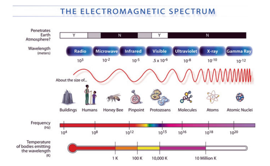
Electromagnetic Spectrum

- Various imaging techniques exploit different parts of the EM spectrum.

---

Chapter 2: Transmission Imaging – X-RaysX-Ray Imaging Basics

- Planar radiography and CT based on X-ray attenuation through tissue.

- Detector measures intensity after passing through body.

Photon-Tissue Interactions

- Photoelectric effect:

- Photon fully absorbed by inner-shell electron → ionization → DNA damage risk.

- Compton scattering:

- Partial energy transfer to outer electron → scattered photon contributes to background noise.

- Rayleigh scattering: elastic scattering, small directional change.

- Pair production: at high energies, not relevant for imaging.

Attenuation Model

- Exponential decay:

N = N_0 e^{-\mu x}

- Total attenuation:

\mu = \mu_{\text{photo}} + \mu_{\text{Compton}}

- Line integral for intensity:

I = I_0 \varepsilon(E) e^{-\int \mu dl}

Contrast in X-Ray Imaging

- Arises from differences in attenuation coefficients between tissues.

- Bone has significantly higher attenuation (due to calcium K-edge).

- Soft tissues have very similar attenuation → low contrast.

Scattered Radiation and Background

- Background signal:

I(x, y) = I_{\text{primary}} + I_{\text{secondary}}

- Scatter-to-primary ratio (R) reduces contrast:

C = \frac{1 - e^{-(\mu_1 - \mu_2)\delta}}{1 + R}

Anti-Scatter Grids

- Reduce scatter by absorbing off-angle photons using lead strips.

- Improves contrast but increases dose (less energy reaches detector).

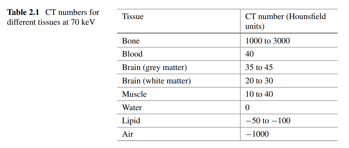
CT Number (Hounsfield Units)

- Relative measure of attenuation:

\text{CT} = 1000 \cdot \frac{\mu - \mu_{\text{H}_2\text{O}}}{\mu_{\text{H}_2\text{O}}}

- Water = 0; air = -1000; bone = 1000–3000.

---

Chapter 3: Reflection Imaging – UltrasoundBasics of Ultrasound

- Mechanical waves (1–10 MHz) need a medium to propagate.

- Transducer:

- Uses piezoelectric material to both emit and receive ultrasound.

Wave Propagation

- Governed by:

\frac{\partial^2 \zeta}{\partial z^2} = \frac{1}{c^2} \frac{\partial^2 \zeta}{\partial t^2}

- Speed of sound:

c = \sqrt{\frac{1}{\rho \kappa}}

- Intensity:

I = \frac{p^2}{\rho c}

- Intensity level (dB):

IL = 10 \log_{10} \left( \frac{I}{I_{\text{ref}}} \right)

### Acoustic Impedance

- Defined as:

Z = \rho c

- Governs how much sound reflects at tissue boundaries.

Reflection and Refraction

- Normal incidence:

- Pressure reflection coefficient:

R_p = \frac{Z_2 - Z_1}{Z_2 + Z_1}

- Small impedance mismatches → weak reflection (most soft tissues).

- Large mismatch (e.g., air/tissue) → strong reflection → need for coupling gel.

Scattering

- From structures ≈ wavelength in size.

- Rayleigh scattering: uniform, frequency-dependent \propto f^4

- Dense scatterers (e.g., RBCs) → useful for blood flow

- Random scatterers → speckle noise

Absorption

- Main type: relaxation absorption (tissue elastic recoil mismatches wave).

- Classical absorption: from molecular friction.

- Absorption increases with frequency.

Attenuation

- Intensity decay:

I(x) = I_0 e^{-\mu x}

- Amplitude decay:

p(x) = p_0 e^{-\alpha x}, \quad \mu = 2\alpha

- Typically:

\mu \propto f^n, \quad n \approx 1

Contrast in Ultrasound

- Based on impedance differences, not attenuation.

- Attenuation is a limiting factor (reduces depth and SNR).

- Higher frequency → better resolution, worse penetration.

Doppler Ultrasound

- Uses Doppler shift to measure blood flow velocity.

- Frequency shift:

f_D \approx \frac{2 f_i v \cos \theta}{c}

- Positive shift = toward transducer, negative = away.

How do signals for medical imaging differ from other biomedical signals?

Medical imaging signals differ as they provide spatially resolved information rather than indirect measures of physiological processes like heart rate and blood pressure.

What are the four categories of signals leading to medical images?

The four categories are:

- Transmission

- Reflection

- Emission

- Resonance

What is the definition of noise in medical imaging?

Noise is an unwanted signal that can arise from various sources, often associated with the measurement process, such as instrument noise. It may also result from motion during imaging.

What is the simplest case model for noise in a measurement?

The measured signal y is modeled as the true signal s plus a noise component e : y = s + e .

How is noise typically characterized in the simplest model?

Noise is often assumed to be a random value drawn from a normal distribution with zero mean and a standard deviation \sigma : e\sim N(0,\sigma^2) .

What is the equation for signal-to-noise ratio (SNR)?

The SNR is defined as the ratio between the signal magnitude and the noise magnitude: \text{SNR} = \frac{s}{\sigma} .

(denominator is standard deviation, which is root of variance)

How can noise be reduced when making multiple measurements?

If N measurements are made, the noise reduces (and the SNR increases) by a factor of \sqrt{N} .

What types of noise models may deviate from the white noise assumption?

Some processes exhibit coherent noise where there is correlation in noise across time or space, such as speckle in ultrasound images.

What is the mathematical proof showing that the Signal-to-Noise Ratio (SNR) improves by a factor of \sqrt{N} when N independent measurements are averaged?

1. Model Definition: The measured value y can be modeled as:

y = s + e,

where s is the true signal and e is the noise, assumed to follow a normal distribution:

e \sim N(0, \sigma^2).

2. Averaging N Independent Measurements:

Suppose N independent measurements y_i are taken. The average is defined as:

\hat{y} = \frac{1}{N} \sum_{i=1}^{N} y_i.

Substituting y_i = s + e_i , where e_i are independent noise terms:

\hat{y} = \frac{1}{N} \sum_{i=1}^{N} (s + e_i).

3. Separating Signal and Noise:

Using linearity of summation:

\hat{y} = s + \frac{1}{N} \sum_{i=1}^{N} e_i.

Here, \frac{1}{N} \sum_{i=1}^{N} e_i is the averaged noise component.

4. Expected Value of the Averaged Noise:

The expectation of \frac{1}{N} \sum_{i=1}^{N} e_i is:

\mathbb{E} \left[ \frac{1}{N} \sum_{i=1}^{N} e_i \right] = \frac{1}{N} \sum_{i=1}^{N} \mathbb{E}[e_i] = 0,

because each noise term e_i has zero mean.

5. Variance of the Averaged Noise:

The variance of \frac{1}{N} \sum_{i=1}^{N} e_i is:

\text{Var} \left( \frac{1}{N} \sum_{i=1}^{N} e_i \right) = \frac{1}{N^2} \sum_{i=1}^{N} \text{Var}(e_i).

Since e_i are independent and have the same variance \sigma^2 (summation adds the extra N):

\text{Var} \left( \frac{1}{N} \sum_{i=1}^{N} e_i \right) = \frac{1}{N^2} \cdot N \cdot \sigma^2 = \frac{\sigma^2}{N}.

Therefore, the standard deviation of the averaged noise is:

\sigma_{\text{avg}} = \frac{\sigma}{\sqrt{N}}.

6. Signal-to-Noise Ratio (SNR):

For a single measurement, the SNR is:

\text{SNR}_{\text{single}} = \frac{s}{\sigma}.

For N averaged measurements, the SNR becomes:

\text{SNR}_{\text{avg}} = \frac{s}{\sigma_{\text{avg}}} = \frac{s}{\sigma / \sqrt{N}} = \sqrt{N} \cdot \frac{s}{\sigma}.

7. Conclusion:

The SNR improves by a factor of \sqrt{N} when N independent measurements are averaged:

\text{SNR}_{\text{avg}} = \sqrt{N} \cdot \text{SNR}_{\text{single}}.

What is the definition of contrast (C_{AB}) in medical imaging?

C_{AB} = |S_A - S_B|, where S_A and S_B represent the signals from different objects or tissues.

How is the normalized contrast (C_{AB}) calculated?

The normalized contrast is calculated as:

C_{AB} = \frac{|S_A - S_B|}{S_A}.

What is the formula for the Contrast-to-Noise Ratio (CNR)?

The CNR is given by:

CNR_{AB} = \frac{C_{AB}}{\sigma},

where \sigma is the standard deviation of the noise.

How can the CNR (CNR_{AB}) be expressed in terms of the SNRs of two tissues (SNR_A and SNR_B)?

Using the definitions of CNR_{AB} and SNR, it can be shown that:

CNR_{AB} = |SNR_A - SNR_B|.

What is the implication of CNR_{AB} = |SNR_A - SNR_B| for achieving a good CNR?

Achieving a good CNR depends on having a sufficiently large difference between the SNRs of the two tissues being compared. If the SNRs of the tissues are very close, the CNR will be low, making it harder to distinguish between them.

Electromagnetic spectrum

What is the primary principle behind transmission-based medical imaging systems like X-rays?

Transmission imaging records the differential transmission of electromagnetic waves (such as X-rays) through the body to generate an image.

What are X-rays commonly used for in medical imaging, and what advanced technique is derived from them?

X-rays are commonly used for planar radiography, such as imaging broken bones. An advanced 3D imaging technique derived from X-rays is computed tomography (CT).

How are X-rays generated and detected in a medical imaging system?

X-rays are generated by high-energy electrons striking a metal target in an evacuated tube. They pass through the body and are detected by converting the X-rays into visible light, which is then transformed into a voltage signal.

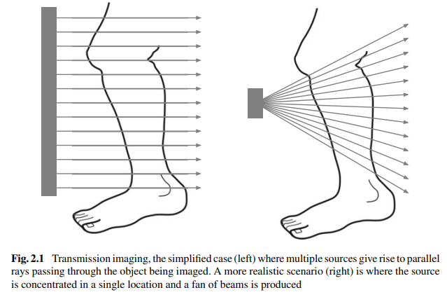
What is the difference between a simplified transmission imaging setup and a realistic one?

In the simplified case, multiple sources generate parallel rays passing through the object. In a realistic scenario, the source is concentrated in a single location, producing a fan of beams.

What is photoelectric attenuation in X-ray imaging?

Photoelectric attenuation is the absorption of X-rays when an incident photon interacts with an atom, causing a tightly bound electron to be emitted and the X-ray energy to be completely absorbed.

An electron from a higher energy level fills the "hole" left by the emitted electron, releasing energy that is absorbed elsewhere in the tissue, resulting in the complete absorption of the X-ray photon.

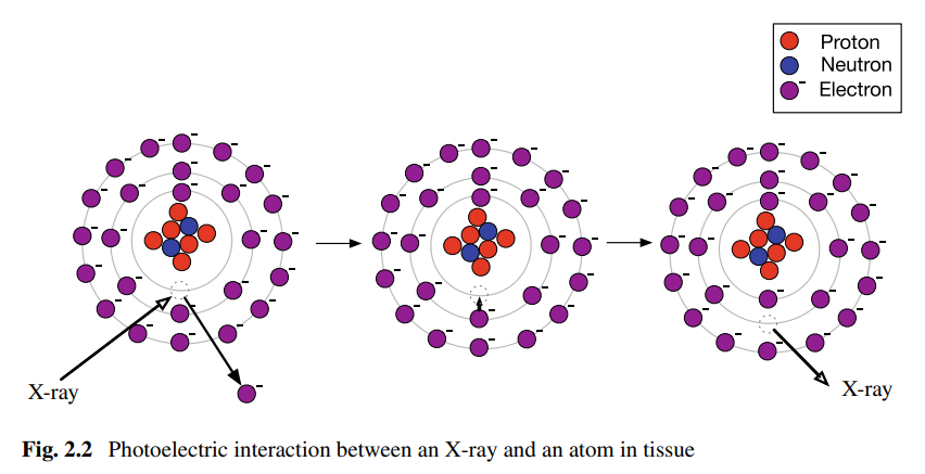
Why are X-rays considered ionizing radiation?

X-rays create ions by ejecting electrons from atoms during the photoelectric attenuation process, which can lead to cell damage and DNA mutation, increasing the risk of cancer.

Why is the dose of X-ray radiation strictly limited in medical imaging?

Due to the ionizing nature of X-rays, prolonged or repeated exposure can cause cell damage and increase the risk of developing cancer. Therefore, the quantity and frequency of X-ray exposure are tightly controlled.

What is Compton scattering in the context of X-ray imaging?

Compton scattering occurs when an X-ray photon interacts with loosely bound electrons in the outer shell of an atom, transferring some energy to the electron and causing the photon to be deflected from its original path.

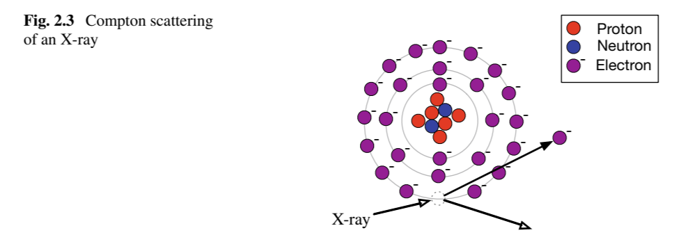
Why is Compton scattering considered a form of attenuation?

The deflected X-ray photon no longer reaches the detector directly opposite the source, reducing the intensity of the detected signal along that path.

How does Compton scattering affect the image quality in X-ray imaging?

The deflected photons can still be detected, but they contribute as an extra "background" signal, reducing the contrast and quality of the final image.

What is the attenuation coefficient ( \mu ) in X-ray imaging?

The attenuation coefficient ( \mu ) describes the rate at which X-rays are absorbed or scattered as they pass through tissue, combining contributions from photoelectric and Compton effects:

\mu(E) = \mu_{\text{photo}}(E) + \mu_{\text{Compton}}(E).

What is the equation for the transmitted intensity of X-rays through a tissue of thickness x ?

For N_0 incident X-rays, the number transmitted, N, through tissue of thickness x is:

N = N_0 e^{-\mu x},

where \mu is the attenuation coefficient.

How is the attenuation of X-rays typically characterized?

Attenuation is often expressed as the mass attenuation coefficient ( \mu/\rho ) in units of \text{cm}^2 \text{g}^{-1} , which normalizes \mu by the tissue density \rho .

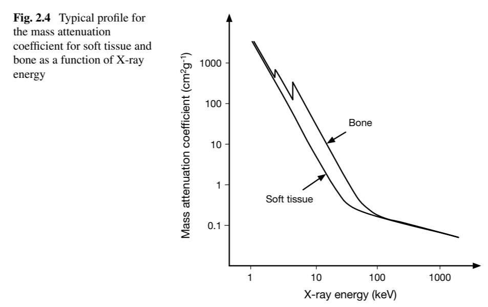
How does the X-ray energy affect the attenuation coefficient for soft tissue and bone?

As the energy of the X-ray increases, the attenuation coefficient decreases for both soft tissue and bone, with bone having a higher attenuation coefficient than soft tissue across the energy spectrum.

What is the equation for the intensity of X-rays measured at a detector after passing through an object with varying attenuation?

The intensity is given by:

I = I_0 \epsilon(E) e^{-\int \mu dl},

where \epsilon(E) is the detector's sensitivity to X-ray energy E and the integral accounts for the cumulative attenuation along the path.

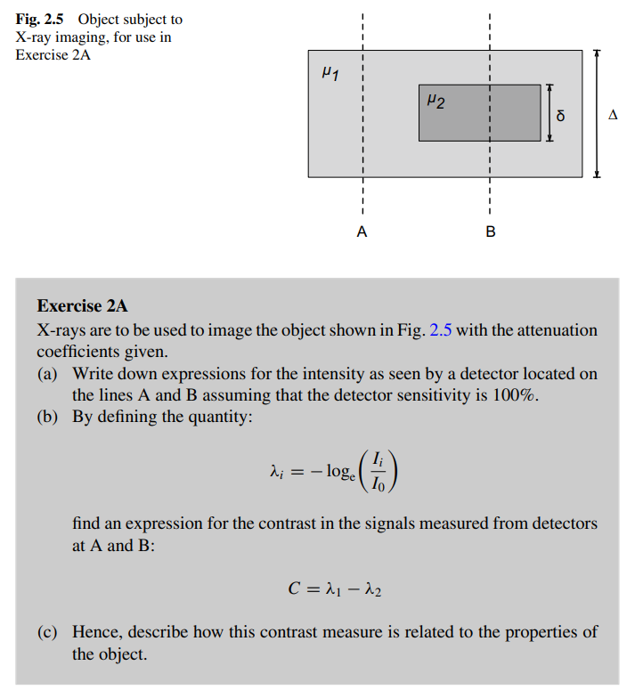
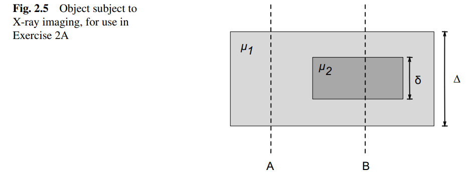
How is the contrast between two signals in X-ray imaging calculated, and how is it related to the object's properties?

1. Intensity Expressions: The intensity at detectors A and B, assuming 100% detector sensitivity, can be expressed as:

I_A = I_0 e^{-\mu_1 \Delta}

I_B = I_0 e^{-\mu_1 (\Delta - \delta)} e^{-\mu_2 \delta},

where I_0 is the initial intensity, \mu_1 and \mu_2 are the attenuation coefficients of the two regions, \Delta is the total thickness, and \delta is the thickness of the inner object.

2. Defining \lambda_i : The quantity \lambda_i is defined as:

\lambda_i = -\ln \left( \frac{I_i}{I_0} \right).

For detectors A and B:

\lambda_1 = \mu_1 \Delta

\lambda_2 = \mu_1 (\Delta - \delta) + \mu_2 \delta.

3. Contrast Formula: The contrast C is given by:

C = \lambda_1 - \lambda_2 = \delta (\mu_2 - \mu_1).

4. Relation to Object Properties: The contrast depends on the difference in attenuation coefficients ( \mu_2 - \mu_1 ) and the thickness ( \delta ) of the inner region. Greater differences in attenuation or a thicker inner region increase the contrast, making it easier to distinguish between the two regions.How is the contrast between two signals in X-ray imaging calculated, and how is it related to the object's properties?

What is the background signal in X-ray imaging, and how does it affect image quality?

The background signal arises from scattered photons that add unhelpful contributions to the detected signal. This reduces the ability to extract useful information about tissue attenuation differences, lowering image quality.

How is the total intensity I(x, y) at a detector calculated in the presence of primary and secondary photons?

The total intensity is:

I(x, y) = I_{\text{primary}}(x, y) + I_{\text{secondary}}(x, y),

where I_{\text{primary}}(x, y) represents photons arriving directly from the source, and I_{\text{secondary}}(x, y) accounts for scattered photons.

What is the equation for primary photon intensity, and what factors does it depend on?

The primary photon intensity is:

I_{\text{primary}}(x, y) = I_0 \epsilon(E, 0) e^{-\int \mu dl},

where I_0 is the initial intensity, \epsilon(E, 0) is the detector efficiency for photons of energy E arriving at an angle \theta = 0 , and \mu is the attenuation coefficient.

What is the explanation of equation 2.6 , which expresses the secondary photon intensity?

Equation 2.6 provides a detailed integral for the secondary photon intensity:

I_{\text{secondary}}(x, y) = \int \int \epsilon(E_s, \theta) E_s S(x, y, E_s, \Omega) \, dE_s \, d\Omega.

Here:

1. Integration over Energy: The outer integral sums over the range of photon energies E_s that the detector is sensitive to.

2. Integration over Solid Angles: The inner integral sums over all directions (solid angle \Omega ) from which scattered photons could arrive at the detector.

3. Components:

- \epsilon(E_s, \theta) : Efficiency of the detector for photons of energy E_s arriving at an angle \theta ,

- E_s : Energy of the scattered photon,

- S(x, y, E_s, \Omega) : Scatter distribution function, representing the number of scattered photons at position (x, y) with energy E_s and direction \Omega .

This equation accounts for the detailed contribution of scattered photons across all energies and directions. However, it is often too complex for practical use and is simplified in approximations like Equation 2.7 .

How is the secondary photon intensity I_{\text{secondary}}(x, y) approximated?

The secondary photon intensity is approximated as:

I_{\text{secondary}}(x, y) = (\bar{\epsilon}_s \bar{E}_s) \bar{S},

where:

- \bar{\epsilon}_s is the average efficiency of the detector,

- \bar{E}_s is the average energy per scattered photon,

- \bar{S} is the number of scattered photons per unit area at the center of the image (assumed to be the worst case).

What is the scatter-to-primary ratio ( R ) and how is the total intensity expressed with it?

The scatter-to-primary ratio R represents the contribution of scattered photons relative to primary photons. The total intensity becomes:

I(x, y) = N \epsilon(E, 0) E (1 + R) e^{-\int \mu dl}.

What is the explanation for the equation I(x, y) = N \epsilon(E, 0) E (1 + R) e^{-\int \mu dl} ?

This equation describes the total intensity at a detector point (x, y) . It combines contributions from primary and scattered photons:

- N : Number of photons emitted from the source.

- \epsilon(E, 0) : Detector efficiency for photons of energy E arriving at an angle of 0°.

- E : Energy of the photons.

- (1 + R) : Accounts for the contribution of scattered photons, where R is the scatter-to-primary ratio.

- e^{-\int \mu dl} : Attenuation of photons along the path, dependent on the attenuation coefficient \mu .

The term (1 + R) separates the contributions of primary photons ( 1 ) and scattered photons ( R ) to the total intensity.

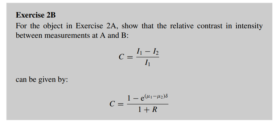
How does the contribution of scattered photons influence contrast, and what are the implications for distinguishing materials?

Steps to Derive Relative Contrast Equation:

1. Relative Contrast Definition:

C = \frac{I_1 - I_2}{I_1},

where I_1 and I_2 are the intensities measured at detectors A and B, respectively.

2. Expressions for Intensities:

Using the attenuation equation I = I_0 e^{-\mu x} , the intensities at A and B are:

I_1 = N \epsilon(E, 0) E e^{-\mu_1 \Delta},

I_2 = N \epsilon(E, 0) E e^{-\mu_1 (\Delta - \delta)} e^{-\mu_2 \delta}.

3. Substitute into Contrast Formula:

Substitute I_1 and I_2 into the contrast equation:

C = \frac{N \epsilon(E, 0) E e^{-\mu_1 \Delta} - N \epsilon(E, 0) E e^{-\mu_1 (\Delta - \delta)} e^{-\mu_2 \delta}}{N \epsilon(E, 0) E e^{-\mu_1 \Delta}}.

4. Simplify the Expression:

Factor out N \epsilon(E, 0) E e^{-\mu_1 \Delta} from the numerator:

C = \frac{1 - \frac{e^{-\mu_1 (\Delta - \delta)} e^{-\mu_2 \delta}}{e^{-\mu_1 \Delta}}}{1}.

Simplify the exponentials:

C = 1 - e^{(\mu_1 - \mu_2) \delta}.

5. Incorporate Scatter ( R ):

The scatter-to-primary ratio R accounts for the contribution of scattered photons relative to the primary photons, which reduces the total intensity contrast. When scatter is included, the total detected intensity is effectively increased due to the added scatter intensity.

Since R represents the scatter-to-primary ratio, the denominator of the contrast formula is adjusted to include (1 + R) , which reduces the overall contrast:

C = \frac{1 - e^{(\mu_1 - \mu_2) \delta}}{1 + R}.

Here’s how R modifies the equation:

- R > 0 : The presence of scattered photons increases the total intensity detected, making the numerator 1 - e^{(\mu_1 - \mu_2) \delta} smaller relative to the total intensity.

- 1 + R : This term explicitly shows the proportion of scattered photons added to the primary intensity, which dilutes the contrast.

What is the purpose of anti-scatter grids in X-ray imaging?

Anti-scatter grids reduce the effect of scattered photons that contribute to background signal, improving contrast between tissues and the background.

How do anti-scatter grids work?

Anti-scatter grids consist of parallel strips of lead foil that absorb photons not arriving within a very tight range of angles, effectively removing a large proportion of scattered X-rays.

What is the trade-off of using anti-scatter grids?

While anti-scatter grids improve contrast by reducing scattered photons, they also reduce the overall received intensity, requiring a larger X-ray dose to achieve adequate imaging, increasing patient exposure.

What is the CT number, and how is it calculated in CT imaging?

The CT number is a dimensionless value that quantifies the attenuation of a material relative to water, used in CT imaging to distinguish different tissues. It is calculated using the formula:

CT = \frac{1000 (\mu - \mu_{\text{H}_2\text{O}})}{\mu_{\text{H}_2\text{O}}},

where:

- \mu : The attenuation coefficient of the material being imaged.

- \mu_{\text{H}_2\text{O}} : The attenuation coefficient of water, used as a reference material.

Key Points:

1. Units: The CT number is measured in Hounsfield units (HU).

2. Range: Typical CT numbers range from -1000 (air) to +3000 (dense bone).

3. Interpretation:

- A CT number of 0 corresponds to water.

- Positive values indicate materials with higher attenuation than water (e.g., bone).

- Negative values indicate materials with lower attenuation than water (e.g., air).

4. Practical Use: This scale allows easy differentiation of tissues in medical imaging, with most tissues having CT numbers similar to water, while bone has the highest CT numbers.

Worked Example:

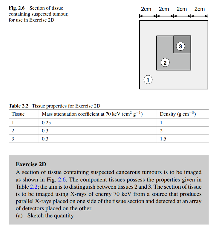
A tissue section containing possible cancer (Fig. 2.6) is made of three tissue types (Table 2.2). The goal is to create a stepwise function that models the attenuation through the section.

The X-rays are parallel and pass through the tissue to detectors on the opposite side.

Type	Description
Mass attenuation coefficient \mu_m (cm²/g)	Material’s x-ray absorption per unit mass
Linear attenuation coefficient \mu = \mu_m \cdot \rho (cm⁻¹)	Absorption per unit distance in the material
Total attenuation \lambda= \mu \cdot \text{distance}	Cumulative absorption along the ray path through the material

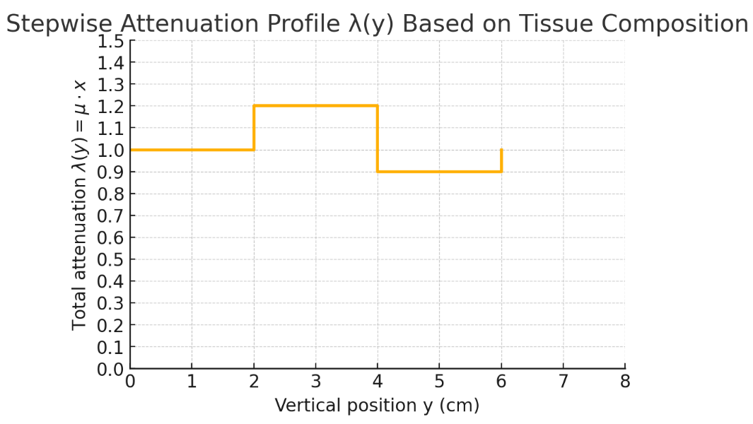
Deriving \lambda(y) as a Function of Position

1. General Expression for \lambda(y) (function of attenuation):

The quantity \lambda(y) is defined as:

\lambda(y) = -\ln\left(\frac{I(y)}{I_0}\right),

=\int\mu dy

Thus:

=\mu x,

where x is the thickness of the material along the path of the X-ray (switched out y for x)

2. Mass Attenuation Coefficients:

For tissues 1, 2, and 3, the linear attenuation coefficient \mu is calculated as:

\mu = (\text{mass attenuation coefficient}) \times (\text{density}).

Using the values provided in Table 2.2:

- For Tissue 1: \mu_1 = 0.25 \times 1 = 0.25 \, \text{cm}^{-1} ,

- For Tissue 2: \mu_2 = 0.3 \times 2 = 0.6 \, \text{cm}^{-1} ,

- For Tissue 3: \mu_3 = 0.3 \times 1.5 = 0.45 \, \text{cm}^{-1} .

3. Thicknesses of Tissues:

From Fig. 2.6:

- Tissue 1 spans 4 \, \text{cm} ,

- Tissue 2 spans 2 \, \text{cm} ,

- Tissue 3 spans 2 \, \text{cm} .

4. Calculating \lambda(y) for Each Region:

For each region along y , \lambda(y) = \mu \times (\text{thickness}) .

- Region Corresponding to Tissue 1:

\lambda_1 = \mu_1 \times 4 = 0.25 \times 4 = 1.0.

- Region Corresponding to Tissue 2:

\lambda_2 = \mu_2 \times 2 = 0.6 \times 2 = 1.2.

- Region Corresponding to Tissue 3:

\lambda_3 = \mu_3 \times 2 = 0.45 \times 2 = 0.9.

Thus, the values of \lambda(y) are:

- 1.0 for Tissue 1,

- 1.2 for Tissue 2,

- 0.9 for Tissue 3.

These values can be sketched as a stepwise function of y , with the positions and values corresponding to the different tissues.

Part B

Part (b): Calculating the Contrast Between Tissues 2 and 3

Contrast Formula:

The relative contrast C between two regions is defined as:

C = \frac{\lambda_2 - \lambda_3}{\lambda_2}.

Substituting the Values:

For Tissues 2 and 3:

- \lambda_2 = 1.2 ,

- \lambda_3 = 0.9 .

C = \frac{1.2 - 0.9}{1.2} = \frac{0.3}{1.2} = 0.25.

Interpretation:

The contrast between Tissues 2 and 3 is 0.25 , indicating a moderate differentiation between the two tissues in terms of attenuation.

---

Final Results:

1. The values of \lambda(y) for the three regions are 1.0 , 1.2 , and 0.9 , respectively, corresponding to Tissues 1, 2, and 3.

2. The contrast C between Tissues 2 and 3 is 0.25 .

Summary so far

Transmission Method

• Noise in Imaging

• Contrast and Contrast-to-Noise Ratio (CNR)

• X-Ray Imaging: Basic Principles

• Attenuation Mechanisms

• Image Intensity and Contrast

• Scattered Radiation and Background

• Anti-Scatter Grids

• CT Imaging and CT Numbers

Forms of attenuation:

• Photoelectric effect: Photon completely absorbed by inner-shell electron → ionization.

• Compton scattering: Photon scatters off outer-shell electron → partial energy loss, background noise.

• Total attenuation: Sum of photoelectric and Compton effects combined.

• Exponential attenuation: Intensity decreases exponentially with thickness.

Moving on to Reflection

What is the principle behind reflection-based medical imaging using ultrasound?

Reflection-based imaging utilizes differences in the acoustic properties of tissues that cause sound waves to reflect at interfaces. These reflections help identify internal structures.

What is ultrasound, and how is it used in medical imaging?

Ultrasound is a mechanical pressure wave that propagates as localized oscillations in pressure, density, and particle velocity. In medical imaging, it operates at frequencies of 1–10 MHz and propagates through tissue as longitudinal waves.

What is the role of a transducer in ultrasound imaging?

The transducer generates ultrasonic waves by converting electrical signals into mechanical oscillations and detects reflections by converting mechanical oscillations back into electrical signals.

What is the wave equation for sound wave propagation in tissue?

The displacement \zeta of a particle as a sound wave propagates is governed by:

\frac{\partial^2 \zeta}{\partial z^2} = \frac{1}{c^2} \frac{\partial^2 \zeta}{\partial t^2},

where c is the speed of sound in the medium.

What determines the speed of sound c in tissue, and what is its approximate value in soft tissues?

The speed of sound c depends on the tissue density \rho_0 and compressibility \kappa , given by:

c = \frac{1}{\sqrt{\rho_0 \kappa}}.

- In soft tissues, c is approximately 1540 \, \text{m/s} .

- Compressibility has units of \text{Pa}^{-1} and is the inverse of the bulk modulus K of the tissue.

- More rigid tissues have a higher bulk modulus and lower compressibility, resulting in a faster speed of sound. Conversely, less rigid tissues have a slower speed of sound.

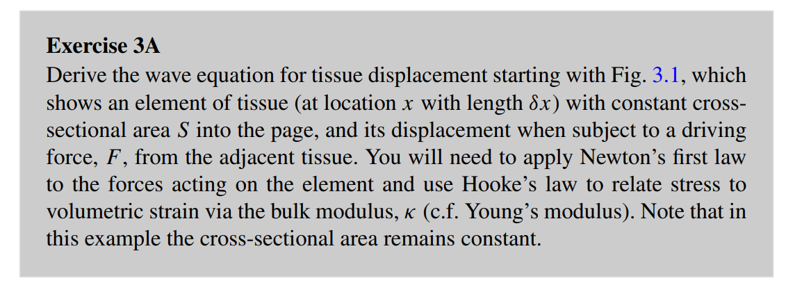
Wave equation derivation

Derivation of the 1D Wave Equation for a Tissue Element

1. Consider the element:

   • Length: \delta x

   • Displacement: \xi(x,t)

   • Force per unit area (stress): F(x,t)

   • Mass density: \rho

   • Cross-sectional area: A

2. Net force on the element (via Taylor expansion):

   • Left side: force = F(x, t)

   • Right side: force = F(x + \delta x, t) = F(x, t) + \frac{\partial F}{\partial x} \delta x

   • Net force:

     \Delta F = \left[F(x + \delta x, t)\right] - F(x, t) = \frac{\partial F}{\partial x} \delta x

3. Apply Newton’s Second Law (Force = mass × acceleration):

   \frac{\partial F}{\partial x} \delta x = \rho A \delta x \frac{\partial^2 \xi}{\partial t^2}

4. Relate force to displacement using Hooke’s Law:

   • Stress is proportional to strain: \text{stress} = E \times \text{strain}

   • Strain = \frac{\partial \xi}{\partial x}

   • Stress = F / A , so:

     \frac{F}{A} = E \frac{\partial \xi}{\partial x} \Rightarrow F = AE \frac{\partial \xi}{\partial x}

   • Differentiate both sides with respect to x :

     \frac{\partial F}{\partial x} = \frac{\partial}{\partial x} \left( AE \frac{\partial \xi}{\partial x} \right)

5. Substitute into Newton’s Law:

   \frac{\partial}{\partial x} \left( AE \frac{\partial \xi}{\partial x} \right) = \rho A \frac{\partial^2 \xi}{\partial t^2}

6. Assume A and E are constant across the material:

   AE \frac{\partial^2 \xi}{\partial x^2} = \rho A \frac{\partial^2 \xi}{\partial t^2}

7. Cancel out A from both sides and simplify:

   E \frac{\partial^2 \xi}{\partial x^2} = \rho \frac{\partial^2 \xi}{\partial t^2}

8. Replace E using compressibility:
   For soft tissues, where bulk modulus K is more appropriate than Young’s modulus E , and noting that:

   \kappa = \frac{1}{K}, \quad \text{and for longitudinal waves in tissue,} \quad E \approx K = \frac{1}{\kappa}

   So:

   \frac{1}{E} \approx \kappa \quad \Rightarrow \quad \frac{\rho}{E} \approx \rho \kappa

   Substituting back:

   \frac{\partial^2 \xi}{\partial x^2} = \rho \kappa \frac{\partial^2 \xi}{\partial t^2}

9. Use wave speed definition c = \frac{1}{\sqrt{\rho \kappa}} :

   \rho \kappa = \frac{1}{c^2}

   So the wave equation becomes:

   \frac{\partial^2 \xi}{\partial x^2} = \frac{1}{c^2} \frac{\partial^2 \xi}{\partial t^2}

What are the wave equations for pressure and particle velocity in a medium?

\frac{\partial^2 \xi}{\partial x^2} = \frac{1}{c^2} \frac{\partial^2 \xi}{\partial t^2}

The wave equations for pressure ( p ) and particle velocity ( u_z ) are:

\frac{\partial^2 p}{\partial z^2} = \frac{1}{c^2} \frac{\partial^2 p}{\partial t^2},

\frac{\partial^2 u_z}{\partial z^2} = \frac{1}{c^2} \frac{\partial^2 u_z}{\partial t^2},

where c is the speed of sound in the medium.

What is D'Alembert's solution to the wave equation?

D'Alembert's solution describes both forward and backward traveling waves as:

p(z, t) = F(z - ct) + G(z + ct),

where F(z - ct) represents the forward-traveling wave, and G(z + ct) represents the backward-traveling wave.

What is the difference between phase velocity and group velocity?

- Phase Velocity: The velocity at which each frequency component of the pulse propagates ( c ).

- Group Velocity: The velocity at which the center of the pulse propagates, evaluated at the center frequency.

What is the equation for intensity ( I ) in a medium?

Intensity is given by:

I = \frac{p^2}{\rho c},

where:

- p is the pressure amplitude (units: Pa, or \text{kg m}^{-1} \text{s}^{-2} ),

- \rho is the medium density (units: \text{kg m}^{-3} ),

- c is the phase velocity (units: \text{m s}^{-1} ).

Intuitive Explanation:

- Pressure Amplitude ( p ): Higher p means more energy in the wave; intensity increases with p^2 .

- Medium Density ( \rho ): Higher \rho means more inertia, which reduces the intensity since the wave has to do more work to move the particles.

- Speed of Sound ( c ): Higher c means the wave energy is spread out more as it propagates faster, so less energy is concentrated per unit area, reducing intensity.

- The formula specifically describes how much energy per unit area per second is carried by the wave for a given pressure amplitude. A higher c spreads this energy across a greater distance in the same time, so less energy is concentrated per unit area (lower I ).

Units Consistency:

The units of I are:

\text{Units of } I = \frac{\text{(Pa)}^2}{\text{kg m}^{-3} \cdot \text{m s}^{-1}} = \frac{\text{kg}^2 \text{m}^{-2} \text{s}^{-4}}{\text{kg m}^{-3} \cdot \text{m s}^{-1}} = \text{W m}^{-2},

which confirms that intensity is measured in watts per square meter.

How is intensity level ( \text{IL} ) in decibels calculated?

Intensity level is calculated as:

\text{IL(dB)} = 10 \log_{10} \left( \frac{I}{I_{\text{ref}}} \right),

where I is the intensity and I_{\text{ref}} is the reference intensity, often 10^{-12} \, \text{W/m}^2 for human hearing at 1 kHz.

What is the relationship between intensity and reflected echoes in ultrasound?

In ultrasound-based medical signals, intensity is most often measured relative to the reflected echoes, comparing the received intensity to the source intensity.

Few key terms

What are bulk modulus ( K ) and compressibility ( \kappa ), and how are they related?

- Bulk Modulus ( K ):

- A measure of a material's resistance to compression.

- Defined as the ratio of pressure change ( \Delta P ) to the relative volume change ( \Delta V / V_0 ):

K = -\frac{\Delta P}{\frac{\Delta V}{V_0}}.

- High K : Material is stiff and resists compression (e.g., steel).

- Units: Pascals ( \text{Pa} ).

- Compressibility ( \kappa ):

- A measure of how easily a material can be compressed.

- Defined as the inverse of the bulk modulus:

\kappa = \frac{1}{K}.

- High \kappa : Material is easily compressible (e.g., air).

- Units: \text{Pa}^{-1} .

How is the speed of sound related to compressibility and density?

The speed of sound in a medium ( c ) depends on how the medium responds to a compressive disturbance, balancing its compressibility ( \kappa ) and density ( \rho ). The relationship is given by:

c = \sqrt{\frac{1}{\rho \kappa}}.

Key Intuitive Concepts:

1. Compressibility ( \kappa ):

- Compressibility measures how easily a material deforms under pressure:

\kappa = \frac{1}{K},

where K is the bulk modulus (stiffness).

- Low Compressibility (High K ): The medium resists compression, causing sound waves to travel faster since the driving force propagates efficiently.

- High Compressibility (Low K ): The medium is easily compressible, absorbing more energy, which slows down the wave.

2. Density ( \rho ):

- Density measures the inertia of the medium, i.e., the mass per unit volume.

- High Density: Particles are harder to accelerate, requiring more energy to move. This slows down the wave.

- Low Density: Particles are easier to accelerate, allowing faster wave propagation.

3. Wave Propagation:

- A sound wave propagates by creating alternating compressions (high pressure) and rarefactions (low pressure) in the medium.

- The wave travels faster in stiff, low-density materials and slower in compressible, high-density materials.

What is the principle behind Doppler ultrasound?

Doppler ultrasound exploits the Doppler effect, which measures changes in frequency of ultrasound waves reflected from a moving object, to calculate velocities.

What is a common application of Doppler ultrasound?

Doppler ultrasound is commonly used to measure blood flow velocity, often using signals scattered from red blood cells (RBCs).

What is the typical size of red blood cells (RBCs), and why is this relevant to Doppler ultrasound?

RBCs are approximately 10 µm in size and densely packed in blood. This small size makes them scatter ultrasound in all directions, resulting in low-intensity backscattered signals received by the transducer.

How does the frequency of ultrasound affect Doppler signal intensity?

The intensity of the Doppler signal is proportional to the fourth power of the ultrasound frequency, so higher frequencies are typically used for blood velocity measurements.

What is the Doppler effect formula for effective incident frequency and reflection frequency in ultrasound?

1. Effective incident frequency ( f_i^{\text{eff}} ):

The frequency perceived by a moving object (e.g., RBCs) when it moves toward or away from the transducer:

f_i^{\text{eff}} = f_i \frac{c + v \cos \theta}{c},

where:

- f_i : Frequency of the incident wave emitted by the transducer,

- c : Speed of sound in the medium,

- v : Velocity of the object (e.g., RBCs),

- \theta : Angle between the direction of object motion and the wave direction.

Explanation: RBC are moving towards the wave at velocity, vcos(theta). The wave is moving towards RBC at velocity, c. The fraction is a ratio of how fast the incident would appear to be moving.

2. Reflection frequency ( f_r ):

The frequency received back at the transducer after the wave reflects off the moving object:

f_r = f_i^{\text{eff}} \frac{c}{c - v \cos \theta}.

Substituting f_i^{\text{eff}} into f_r :

f_r = f_i \frac{c + v \cos \theta}{c - v \cos \theta}.

Explanation: RBC reflect f_i^{\text{eff}}, and the fraction is a ratio between the speed of the actual wave, and the speed perceived by the RCB. This magnified the effective frequency to give the real reflection frequency.

What is acoustic impedance ( Z ), and how is it defined for sound waves?

1. What is Acoustic Impedance?

Acoustic impedance, denoted as Z , describes how much resistance a medium offers to the movement of sound through it. In simpler terms, it tells us how easily or difficultly sound can pass through a material.

2. How is it Defined?

Acoustic impedance is defined mathematically as:

Z = \frac{p}{u_z}

- p : acoustic pressure (i.e., the pressure variation caused by the sound wave)

- u_z : particle velocity in the direction of wave propagation (how fast the particles in the medium move due to the wave)

This formula is a ratio, similar in structure to how we define electrical resistance or impedance.

---

🧠 What This Ratio Represents (Intuitively)

Think of sound as a mechanical wave: it's not an object moving forward, but rather a disturbance that causes particles in the medium (like air or water) to vibrate back and forth.

Imagine This Analogy:

You’re trying to push and pull a sponge back and forth really fast (imitating a sound wave).

- The force you apply is like pressure p

- The speed at which the sponge moves is like particle velocity u_z

- The stiffness or resistance you feel (how hard it is to move it) is like impedance Z

⚙ Breaking Down the Ratio \frac{p}{u_z}

- If it takes a lot of pressure p to produce just a little motion u_z , the impedance is high:

→ The medium is resisting the sound wave strongly.

- If it takes very little pressure to produce a lot of motion, the impedance is low:

→ The medium allows sound to pass through easily.

How does acoustic impedance behave for plane waves?

🔹 1. What Is a Plane Wave?

A plane wave is an idealized sound wave in which:

• The wavefronts (surfaces of constant phase) are infinite, flat planes.

• The wave propagates in a single direction—say, along the zzz-axis—without spreading out.

• Every point on a given wavefront experiences the same pressure and velocity at the same time.

This contrasts with spherical waves (like those from a point source), where the wavefront expands in all directions.

🔹 2. How Does Acoustic Impedance Behave for Plane Waves?

✅ It is Real (Non-Complex)

For plane waves:

Z = \frac{p}{u_z}

- Both p (pressure) and u_z (particle velocity) are in phase—they reach their maximum and minimum at the same time.

- Imagine a sound wave compression passing across a point. Plot the speed of the particles at that point and their pressure against time. The pressure would increase as the way passes through. The speed of the particles would also peak at that same point in time.

- We don’t need imaginary components representing phase differences.

- Therefore, Z is a real number (it has no imaginary part, unlike in many other wave systems).

✅ It is Frequency-Independent

- The impedance does not depend on the wave's frequency.

- This means whether the wave is low-pitched (e.g. 100 Hz) or high-pitched (e.g. 10,000 Hz), the impedance stays the same as long as it’s a plane wave in the same medium.

🔹 3. Why Is This Important?

- In many real-world scenarios (like sound in air ducts or ultrasonic imaging in tissue), approximating waves as plane waves simplifies analysis.

- Since Z is real and frequency-independent, it's a fixed property of the medium—determined only by the medium’s physical properties:

Z = \rho c

where:

- \rho is the medium's density

- c is the speed of sound in that medium

This expression is the characteristic acoustic impedance of the medium.

What is the expression for the characteristic acoustic impedance ( Z ) of a medium?

The characteristic acoustic impedance is given by:

Z = \rho c,

where:

- \rho : Density of the medium (in \text{kg/m}^3 ),

- c : Speed of sound in the medium (in \text{m/s} ).

How do we derive the characteristic acoustic impedance of a medium?

SKIP??

How do we get this? From substituting the following formula:

For a plane wave propagating in a medium, the acoustic pressure p and particle velocity u_z are related by the wave equation. Specifically:

p = \rho c,

where:

- \rho : Density of the medium,

- c : Speed of sound in the medium.

Intuitive Explanation

- The pressure fluctuation p arises from compressions and rarefactions in the medium due to particle motion.

- The density \rho determines the inertia of the particles.

- The speed of sound c relates the temporal and spatial variations of the wave.

- Combining these factors gives p = \rho c , linking the pressure and particle velocity.

This equation shows that pressure is proportional to both the particle velocity and the medium's properties ( \rho and c ).

How can acoustic impedance be related to the compressibility of a medium?

Acoustic impedance can also be expressed in terms of density ( \rho ) and compressibility ( \kappa ) as:

Z = \sqrt{\frac{\rho}{\kappa}}.

Here:

- \kappa : Compressibility, the inverse of bulk modulus ( \text{Pa}^{-1} ).

1. From the speed of sound in a medium (see previous deck):

c = \sqrt{\frac{1}{\rho \kappa}}.

2. Substituting c into Z = \rho c :

Z = \rho \sqrt{\frac{1}{\rho \kappa}} = \sqrt{\frac{\rho}{\kappa}}.

Thus, all three representations are consistent and describe the same property from different perspectives:

- Definition ( Z = p / u_z ) focuses on the wave's dynamic properties.

- Medium-Based ( Z = \rho c ) focuses on the macroscopic properties of the medium.

- Compressibility-Based ( Z = \sqrt{\rho / \kappa} ) focuses on the material's fundamental mechanical properties.

What are the typical units and applications of acoustic impedance?

- Units: \text{kg/m}^2 \, \text{s}^{-1} .

- Applications: Acoustic impedance is crucial for understanding wave transmission and reflection at tissue interfaces in ultrasound and other acoustic systems.

What happens when an ultrasound wave hits a boundary between two tissues with different acoustic properties?

When an ultrasound wave hits a boundary, part of the wave is reflected and part is transmitted, depending on the acoustic properties of the tissues. The behavior is similar to light waves at a boundary:

- The angle of incidence equals the angle of reflection: \theta_i = \theta_r .

- Refraction is governed by Snell's law:

\frac{\sin \theta_i}{\sin \theta_t} = \frac{c_1}{c_2},

where c_1 and c_2 are the speeds of sound in the two tissues.

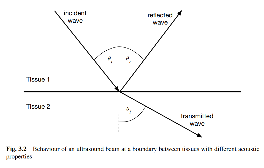
What are the reflection and transmission coefficients for ultrasound waves at a boundary?

- Pressure Reflection Coefficient ( R_p ):

R_p = \frac{Z_2 - Z_1}{Z_2 + Z_1},

where Z_1 and Z_2 are the acoustic impedances of the two tissues.

- Pressure Transmission Coefficient ( T_p ):

T_p = \frac{2Z_2}{Z_2 + Z_1}.

How do we calculate the intensity reflection and transmission coefficients?

- Intensity Reflection Coefficient ( R_I ):

R_I = \left( \frac{Z_2 - Z_1}{Z_2 + Z_1} \right)^2.

- Intensity Transmission Coefficient ( T_I ):

T_I = \frac{4Z_1 Z_2}{(Z_2 + Z_1)^2}.

Why is reflection important in ultrasound imaging?

- Reflection occurs at tissue boundaries due to differences in acoustic impedance.

- Reflections are used to detect boundaries and create images of structures within the body.

- Key Insights:

- If Z_1 = Z_2 : No reflection ( R_I = 0 ).

- If Z_1 or Z_2 approaches 0: Reflection is maximized ( R_I \to 1 ), which prevents deeper penetration of the wave.

Why is a coupling gel used in ultrasound imaging?

- A coupling gel eliminates air between the probe and skin to minimize reflection at the probe-skin interface.

- Without the gel, the large impedance difference between air and tissue would create a strong reflection, preventing the wave from entering the body.

What happens when ultrasound waves strike objects smaller or similar in size to their wavelength?

When ultrasound waves encounter objects that are similar in size or smaller than their wavelength, they scatter in all directions. The intensity of scattering depends on the object's shape, size, and acoustic properties.

What is Rayleigh scattering, and when does it occur in ultrasound imaging?

Rayleigh scattering occurs when the scatterer is very small compared to the ultrasound wavelength. It produces relatively uniform scattering in all directions, with slightly more energy scattered backward. The scattered energy increases with the fourth power of frequency.

How does scattering contribute to ultrasound blood flow measurements?

Constructive interference occurs when scatterers, like red blood cells, are densely packed. This constructive scattering enhances ultrasound's ability to measure blood flow.

What is speckle in ultrasound imaging?

Speckle is a type of "noise" in ultrasound images caused by widely spaced, randomly distributed scatterers. This noise can reduce the clarity of the image.

What causes absorption of ultrasound waves in tissues?

Absorption occurs when ultrasound energy is lost as it propagates through tissue. This energy loss happens due to:

1. Relaxation absorption: Energy is lost as tissue returns to its equilibrium position.

2. Classical absorption: Caused by friction between particles within the tissue.

How does absorption work in ultrasound imaging?

Absorption occurs when ultrasound waves pass through tissue and lose energy due to the following process:

- As the ultrasound wave displaces tissue, the tissue experiences elastic restoring forces that pull it back to equilibrium.

- Energy loss occurs depending on how well the wave's frequency matches the tissue's relaxation time:

- If the relaxation matches the wave's force, little energy is lost because both forces act in the same direction.

- If they don't match, more energy is lost as the wave forces the tissue away from equilibrium while the tissue tries to return.

- Another mechanism of absorption is classical absorption, caused by friction between particles in the tissue, with energy loss proportional to f^2 .

What is relaxation absorption in ultrasound?

Relaxation absorption occurs when tissue displaced by ultrasound waves experiences elastic restoring forces. The energy lost depends on the match between the ultrasound frequency ( f ) and the tissue relaxation frequency ( f_r ). This process can be characterized by the absorption coefficient:

\beta_r = \frac{\beta_0 f^2}{1 + \left( \frac{f}{f_r} \right)^2}.

What happens when the tissue relaxation frequency matches the ultrasound wave frequency?

When the tissue relaxation frequency ( f_r ) matches the ultrasound wave frequency ( f ), very little energy is absorbed. If they do not match, more energy is lost, leading to greater attenuation of the ultrasound wave.

What is classical absorption in ultrasound imaging?

Classical absorption is caused by friction between particles in the tissue. The absorption in this case is proportional to the square of the ultrasound frequency.

Why is absorption important in ultrasound imaging?

Absorption reduces the intensity of ultrasound waves as they propagate through tissues. It contributes to attenuation alongside reflection and scattering, impacting the depth and quality of the imaging.

What are the three ways ultrasound waves are attenuated in tissue?

Ultrasound waves lose intensity as they travel through tissue due to:

1. Reflection (useful): Part of the wave reflects back at boundaries between tissues with different acoustic impedances.

• The reflection is what allows the machine to receive a signal and assign a position to a structure in the body. The attenuation is the limited amount that is reflected.

• The amount (intensity) of reflection tells us about the nature of the tissue—specifically, the difference in acoustic impedance between adjacent tissues. This affects how bright or dark that area appears on the image (echogenicity).

2. Scattering: The wave scatters in all directions when encountering objects similar in size to its wavelength.

3. Absorption: Energy is lost as the wave displaces tissue and the tissue resists, returning to equilibrium. This includes:

• Relaxation absorption, which depends on tissue elasticity and wave frequency.

• Classical absorption, caused by friction between particles.

What is the general law for intensity attenuation in a uniform tissue?

The intensity of an ultrasound wave at a point x in a uniform tissue is given by:

I(x) = I_0 e^{-\mu x},

where:

- I(x) : Intensity at distance x ,

- I_0 : Initial intensity,

- \mu : Intensity attenuation coefficient of the tissue.

How is attenuation expressed when the wave passes through tissue with varying attenuation coefficients?

When attenuation varies along the wave's path, the intensity is calculated using an integral:

I = I_0 e^{-\int \mu dl},

where the integral accumulates the effects of attenuation along the path.

What are the units and conversions for the attenuation coefficient ( \mu )?

The attenuation coefficient is typically expressed in units of:

- nepers per cm ( \text{nepers cm}^{-1} ) for natural logarithms (base e ).

- decibels per cm ( \text{dB cm}^{-1} ) for base-10 logarithms.

What do these mean?

➤ Nepers (standard) (Np/cm)

- These are the units we typically use.

- Given the wave model as:

A(x) = A_0 e^{-\mu x}

we can rearrange to make \mu the subject:
\mu = -\frac{1}{x} \ln\left(\frac{A(x)}{A_0}\right)

What does this tell us?

\frac{A(x)}{A_0} is the ratio of attenuation.

then \mu is “how many "natural log units" of amplitude are lost per cm.” This is nepers per cm and it based on natural logarithms (base e ).

➤ Decibels (dB/cm)

- Converting a ratio to decibels tells us about the “gain” of a system.

- Given the ratio of attenuation, we can have a “gain” dB version of attenuation:

\text{Attenuation} = 10 \log_{10} \left(\frac{A_0}{A(x)}\right)

so the decibel form reflects amplitude loss using base-10 logs.

Conversion between these units (derived next card):

\mu[\text{dB cm}^{-1}] = 4.343 \mu[\text{nepers cm}^{-1}].

How is intensity attenuation in tissue similar to X-ray attenuation?

The equation I = I_0 e^{-\mu x} used for ultrasound attenuation is the same model used for X-ray attenuation, where the attenuation coefficient ( \mu ) quantifies energy loss due to scattering and absorption in both cases.

What is the relationship between intensity attenuation coefficient and amplitude attenuation coefficient, and how do they relate in dB cm^{-1}?

(a) Derive the relationship between intensity attenuation in dB cm^{-1}:

1. The intensity attenuation equation is:

I(x) = I_0 e^{-\mu x}.

2. Convert this to decibels using base-10 logarithms:

I[\text{dB}] = 10 \log_{10} \left( \frac{I(x)}{I_0} \right).

dB show a rate of gain/loss. We divide by initial intensity as we want to represent the loss ratio in decibels.

3. Substituting I(x) = I_0 e^{-\mu x} :

I[\text{dB}] = 10 \log_{10} \left( e^{-\mu x} \right).

4. Using \log_{10}(e^a) = a \cdot \log_{10}(e) and \log_{10}(e) \approx 0.4343 :

I[\text{dB}] = -10 \mu x \cdot 0.4343.

5. Simplify to:

\mu[\text{dB cm}^{-1}] = 4.343 \mu[\text{nepers cm}^{-1}].

(b) Express attenuation in terms of pressure amplitude:

1. The pressure amplitude attenuation equation is:

p(x) = p_0 e^{-\alpha x},

where \alpha is the amplitude attenuation coefficient.

2. The intensity I(x) is proportional to the square of the pressure p(x) . From the equation:

I = \frac{p^2}{\rho c},

we know that I \propto p^2 (since \rho and c are constants for a given medium).

3. Substitute p(x) = p_0 e^{-\alpha x} :

I(x) \propto \left( p_0 e^{-\alpha x} \right)^2 = p_0^2 e^{-2\alpha x}.

4. Comparing this with I(x) = I_0 e^{-\mu x} , we see:

\mu = 2\alpha.

(c) Show equivalence in dB cm^{-1}:

1. In dB cm^{-1}, the amplitude attenuation is:

\alpha[\text{dB cm}^{-1}] = 20 \log_{10} \left( e^{-\alpha x} \right) = 4.343 \alpha.

2. For intensity, using \mu = 2\alpha :

\mu[\text{dB cm}^{-1}] = 4.343 \mu = 4.343 (2\alpha) = 4.343 \alpha.

3. Thus, \alpha[\text{dB cm}^{-1}] = \mu[\text{dB cm}^{-1}] .

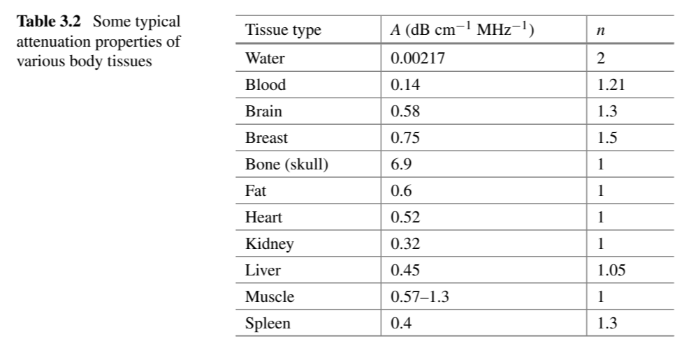
What is the relationship between attenuation coefficient and frequency in biological tissues?

The attenuation coefficient \mu (in dB cm^{-1}) varies with frequency according to the model:

\mu(\text{dB cm}^{-1}) = A f^n,

where:

- A is a proportionality constant,

- f is the frequency of the wave,

- n is an exponent describing the relationship between attenuation and frequency.

Key Insight:

- For most biological tissues, the relationship is approximately linear:

- n \approx 1 ,

- A \approx 1 .

This means attenuation increases roughly linearly with frequency for typical biological tissues.

What are the key properties of tissues that influence ultrasonic imaging?

The following tissue properties impact ultrasonic imaging:

1. Speed of Sound: Determines how quickly the wave propagates through the tissue and affects timing and resolution.

2. Impedance: Differences in impedance at tissue interfaces cause reflections, which generate contrast in reflection-based techniques.

3. Attenuation: Reduces the intensity of the signal due to scattering and absorption, limiting depth penetration and imaging quality.

Why is impedance contrast important in ultrasonic imaging?

Impedance contrast allows reflection-based imaging techniques to work:

1. Reflected signals at tissue interfaces are caused by differences in impedance between the two tissues.

2. The magnitude of reflected signals provides contrast, helping differentiate between tissues.

3. Impedance mismatches are critical for generating meaningful reflections and producing accurate images.

Why is attenuation considered a limitation in ultrasonic imaging?

Attenuation creates challenges in ultrasonic imaging:

1. It reduces the signal magnitude, especially for deeper structures, without adding meaningful tissue information.

2. High attenuation prevents transmission approaches for most body parts, as tissues are too thick for ultrasound to pass through effectively.

3. Attenuation limits depth penetration, necessitating the use of lower frequencies (e.g., 2 MHz) for imaging deep structures like the abdomen.

How does attenuation limit imaging depth in ultrasonic imaging?

Attenuation limits imaging depth due to the following:

1. The attenuation coefficient increases with frequency, causing higher frequencies to lose intensity more quickly.

2. For deeper imaging (e.g., the abdomen), lower frequencies (e.g., 2 MHz) must be used to ensure the wave can penetrate sufficiently.

3. Lower frequencies reduce resolution, creating a trade-off between depth penetration and image clarity.

Recap so far

Transmission Method

• Noise in Imaging

• Contrast and Contrast-to-Noise Ratio (CNR)

• X-Ray Imaging: Basic Principles

• Attenuation Mechanisms

• Image Intensity and Contrast

• Scattered Radiation and Background

• Anti-Scatter Grids

• CT Imaging and CT Numbers

Forms of attenuation:

• Photoelectric effect: Photon completely absorbed by inner-shell electron → ionization.

• Compton scattering: Photon scatters off outer-shell electron → partial energy loss, background noise.

• Total attenuation:

  Sum of photoelectric + Compton effects combined.

• Exponential attenuation: Intensity decreases exponentially with thickness.

---

Moving on to Reflection (Ultrasound)

Speed of Sound

• Reflection occurs due to differences in acoustic properties between tissues.

• Wave Equation:

  \frac{1}{c^2} \frac{\partial^2 \zeta}{\partial t^2} = \frac{\partial^2 \zeta}{\partial x^2}

  where c is the speed of sound.

• Wave Intensity

  I = \frac{p^2}{\rho c}

• Speed of Sound in Tissue

  c = \sqrt{\frac{1}{\rho\kappa}}

• General solution for 1D wave propagation:

  p(z,t) = F(z-ct) + G(z+ct)

Acoustic Impedance

• Acoustic impedance (Z) in ultrasound is the measure of a material's resistance to the propagation of sound waves

  Z = \rho c

• Reflection coefficient R_p (pressure):

  R_p = \frac{Z_2 - Z_1}{Z_2 + Z_1}

• Transmission coefficient T_p :

  T_p = \frac{2Z_2}{Z_1 + Z_2}

Attenuation Properties

Scattering

• Scattering in Ultrasound

• Occurs when wave interacts with small objects (e.g., red blood cells).

• Rayleigh scattering: Scattering intensity \propto f^4 .

• Speckle: Noise-like appearance from random scatterers.

• Doppler effect used to measure blood flow velocity.

• Doppler frequency shifts:

  f_r = f_i \left( \frac{c - v\cos\theta}{c + v\cos\theta} \right)

Intensity Attenuation

• Intensity attenuation:

  I(x) = I_0 e^{-\mu x}

• Attenuation coefficient takes all factors into account. You can also calculate each attenuation cause individually.

• Causes:

  • Reflection

  • Scattering

  • Absorption

    • Relaxation and Classical Friction

• Absorption depends on frequency:

  \beta(f) = \beta_r \frac{1}{1 + (f_r/f)^2}

• Amplitude and intensity attenuation are related:

  • Intensity attenuation coefficient \mu

  • Amplitude attenuation coefficient \alpha

    \mu = 2\alpha

Final Points

- Attenuation limits depth (lower frequencies needed for deeper imaging).

- Trade-off between resolution (higher frequency) and penetration (lower frequency).

- X-ray: Contrast based on attenuation.

- Ultrasound: Contrast based on impedance mismatches and reflected signals.