descriptive statistics

lock in part2

descriptive statistics

• describe what has transpired = stats from the past

• descriptive measures derived from a sample (statistics) and population (parameters) 

three main characteristics used for the numerical description of data?

Center, variability, and shape

Center

(average, middle, most common)

Variability

(how spread out the data is)

Shape

(symmetry, skewness, tails)

Measure of center: Mean

average

• uses all data 

• sensitive to outliers 

Measure of center: median

middle value

• good if outliers exist

If 𝑛 is odd → middle value.

If 𝑛 is even → average of the two middle values.

Measure of center: mode

most frequent value

• good for categories/ discrete data 

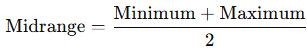
Measure of center: midrange

(max + min) div 2

• easy but distorted by outliers

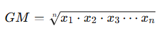
Measure of center: geometric mean

• average of products/ ratio 

• multiply all values 

• take the n-th root 

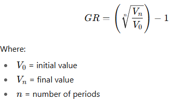
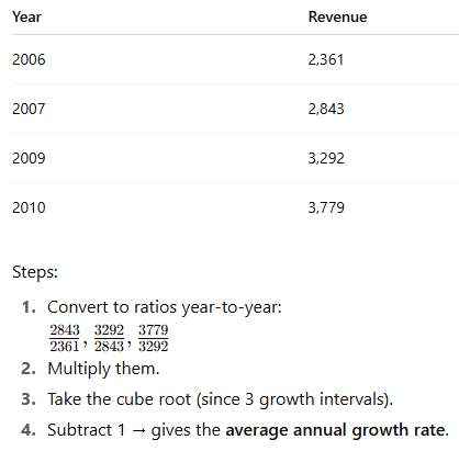
growth rate using geometric mean

• measure of center but best for ratio, percent, growth

• special use of geometric mean to find average rate of change across time 

arithmetic mean (normal ave)

+ all numbers then div number of items 

measure of center 

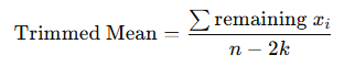
Measure of center: trimmed mean

average after removing extreme high/low values

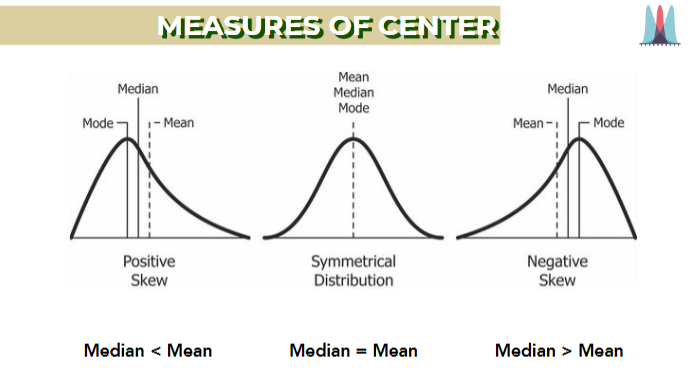
Measure of center

• positive Right-skew: Mean > Median > Mode

• normal Normal: Mean = Median = Mode

• negative Left-skew: Mean < Median < Mode

Measure of Variability: range

diff between largest & smallest observation

• sensitive to data values but ez to interpret

max - min

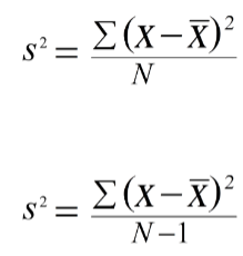
Measure of Variability: sample variance

average of squared deviations (how far a data value is from mean) from mean

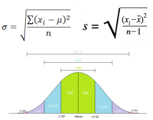
Measure of Variability: standard deviation

• spread of data around mean

• most common same unit as data

• symbol: σ

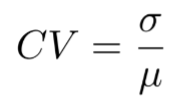
Measure of Variability: coefficient of variations 

• CV = SD div mean x 100%

• compares spread across datasets w/ diff units

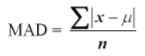
Measure of Variability: mean absolute deviation 

• reveals average distance from center 

• MAD

standardized data

rescale data so everything is measured in terms of how far it is from the mean, using the standard deviation as the unit.

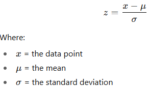
z-score

• z-score says how many standard deviations away from the mean a data point is. = how far from average, in standard deviation units

• Positive z → above the mean.

• Negative z → below the mean.

Helps spot unusual data:

• |z| > 2 → unusual

• |z| > 3 → outlier

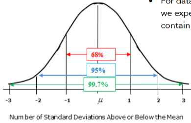
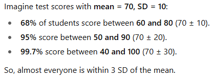
empirical rule

describes how data is spread out in a normal distribution (bell curve)

• ±1 standard deviation from the mean → about 68% of the data falls here.

• ±2 standard deviations from the mean → about 95% of the data falls here.

• ±3 standard deviations from the mean → about 99.7% of the data falls here.

It helps you predict where most data will fall.

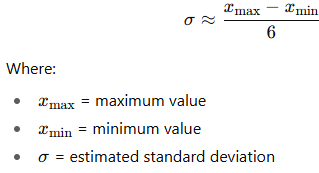
estimating sigma

fast estimate of SD if the data is roughly normal and you only know the min & max.

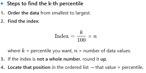
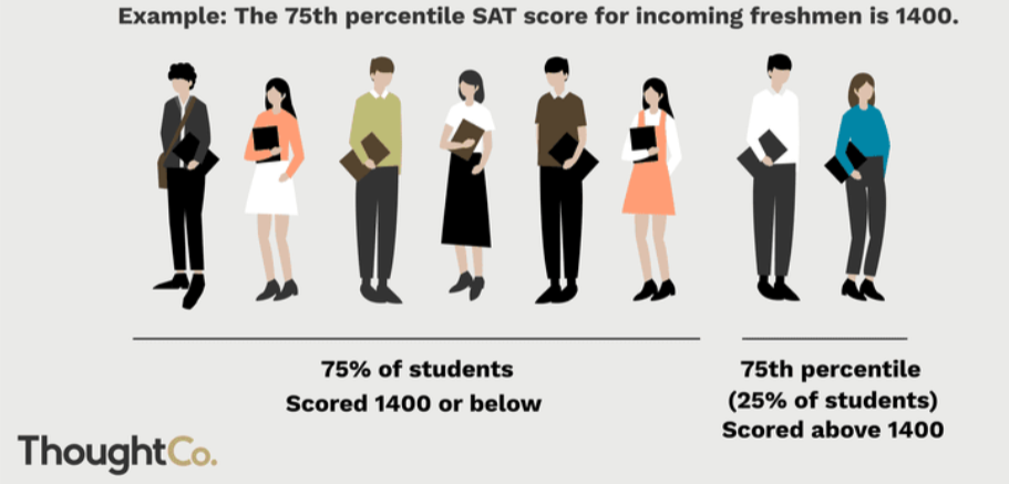
percentiles

position of a value in data

ex: 90th percentile

often used for national edu tests 

quartiles

scale points that div sorted data into 4 grps of equal size

• Q1 (First Quartile) = 25th percentile → 25% of data is below it.

• Q2 (Second Quartile) = 50th percentile = Median → half the data is below it.

• Q3 (Third Quartile) = 75th percentile → 75% of data is below it.

Interquartile Range (IQR) IQR=Q3−Q1

• Show center (Q2) and spread (Q1, Q3).

• Help detect outliers using fences:

  • Lower Fence = Q1−1.5(IQR)

  • Upper Fence = Q3+1.5(IQR)

  • Any data outside = outlier.

Methods for Finding Quartiles

• Method of Medians:

  • Find Q2 (median) first.

  • Q1 = median of lower half.

  • Q3 = median of upper half.

• Interpolation Method:

  • Uses formulas when data size doesn’t split evenly.

box plots

simple graph shows dataset’s center, spread, and skewness using five key numbers:

1. Minimum (smallest value, not an outlier)

2. Q1 (25th percentile)

3. Median (Q2) (50th percentile)

4. Q3 (75th percentile)

5. Maximum (largest value, not an outlier)

= 5-number summary.

How to Read a Boxplot

• The box = middle 50% of the data (from Q1 → Q3).

• The line inside the box = the median (Q2).

• The “whiskers” extend to the smallest and largest values within the fences (not outliers).

• Any points beyond whiskers = outliers.

Fences (for detecting outliers)

• Lower Fence = Q1 – 1.5 × IQR

• Upper Fence = Q3 + 1.5 × IQR

• Outliers are values outside these fences.

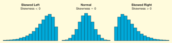
Shape of Distribution

• Skewness = symmetry.

  • Right-skewed: tail on right.

  • Left-skewed: tail on left.

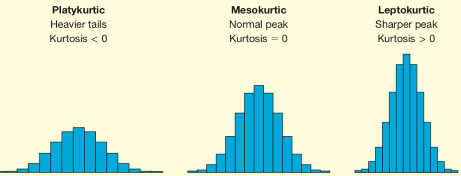
• Kurtosis = tail heaviness & peak.

  • High kurtosis = heavy tails (outliers likely).

  • Low kurtosis = flat distribution.