Chapters on Externalities, Costs, and Consumer Choice

Externality

A cost or benefit of an activity that affects third parties who did not choose to incur that cost or benefit.

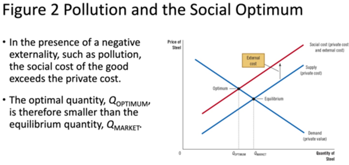
Negative Externality

Leads to overproduction (e.g., pollution).

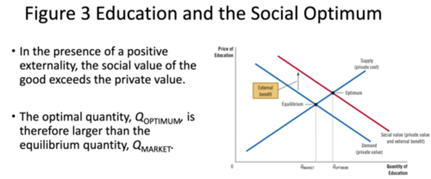
Positive Externality

Leads to underproduction (e.g., education).

Social Cost

= Private Cost + External Cost

Social Value

= Private Value + External Benefit

Market Failure

When externalities are present, the market equilibrium is inefficient because the costs or benefits to society are not considered.

Government Intervention

Can correct market inefficiency through taxes and subsidies.

Coase Theorem

Suggests that private negotiations can solve externalities if property rights are well-defined and transaction costs are low.

Total Cost (TC)

The total expenditure by a firm to produce goods and services. = FC + VC

Fixed Costs (FC)

Costs that do not vary with output.

Variable Costs (VC)

Costs that vary with output.

Profit

= Total Revenue - Total Cost

Average Total Cost (ATC)

= TC / Q

Marginal Cost (MC)

= ΔTC / ΔQ

U-Shaped ATC Curve

The ATC curve is typically U-shaped because of economies and diseconomies of scale.

Marginal Revenue (MR)

= ΔTR / ΔQ

Total Revenue (TR)

= P × Q

Average Revenue (AR)

= TR / Q

Short-Run Supply Curve

The firm's short-run supply curve is the portion of its marginal cost curve above the average variable cost (AVC).

Long-Run Supply Curve

In the long run, firms enter or exit the market based on profits. The supply curve is horizontal at the price that equals minimum average total cost (ATC).

Shutdown (Short-Run)

If price (P) is less than AVC, the firm should shut down.

Exit (Long-Run)

If price (P) is less than ATC, firms should exit the market in the long run.

Budget Constraint

Represents all the possible combinations of goods a consumer can afford given their income and the prices of goods.

Slope of the budget constraint

Slope = P_x / P_y

Indifference Curves

Show combinations of two goods that provide the consumer with the same level of satisfaction.

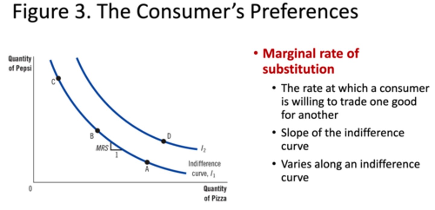
Marginal Rate of Substitution (MRS)

The rate at which a consumer is willing to trade one good for another while staying on the same indifference curve. = MU_x / MU_y

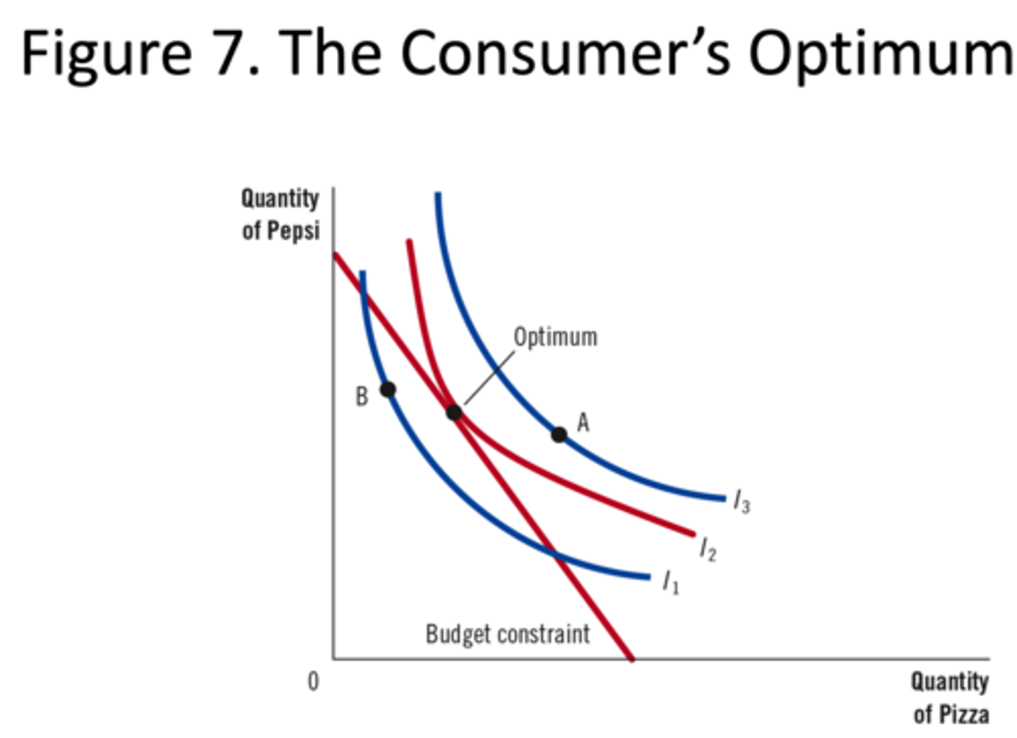
Consumer's Optimum

Occurs where the budget constraint is tangent to the highest indifference curve. MU_x / P_x = MU_y / P_y

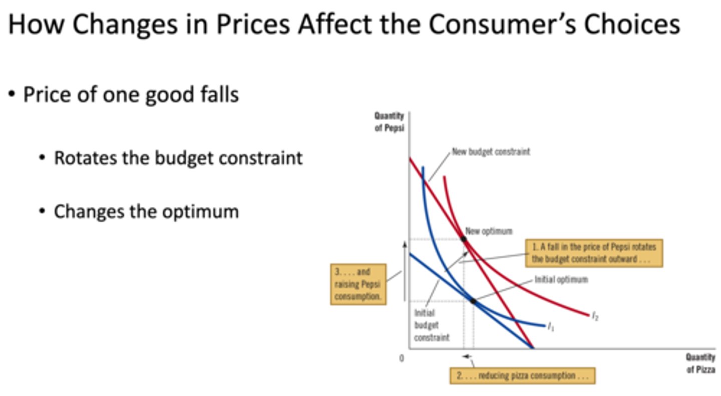
How Changes in Prices Affect the Consumer's Choices

Price of one good falls

• Rotates the budget constraint

• Changes the optimum

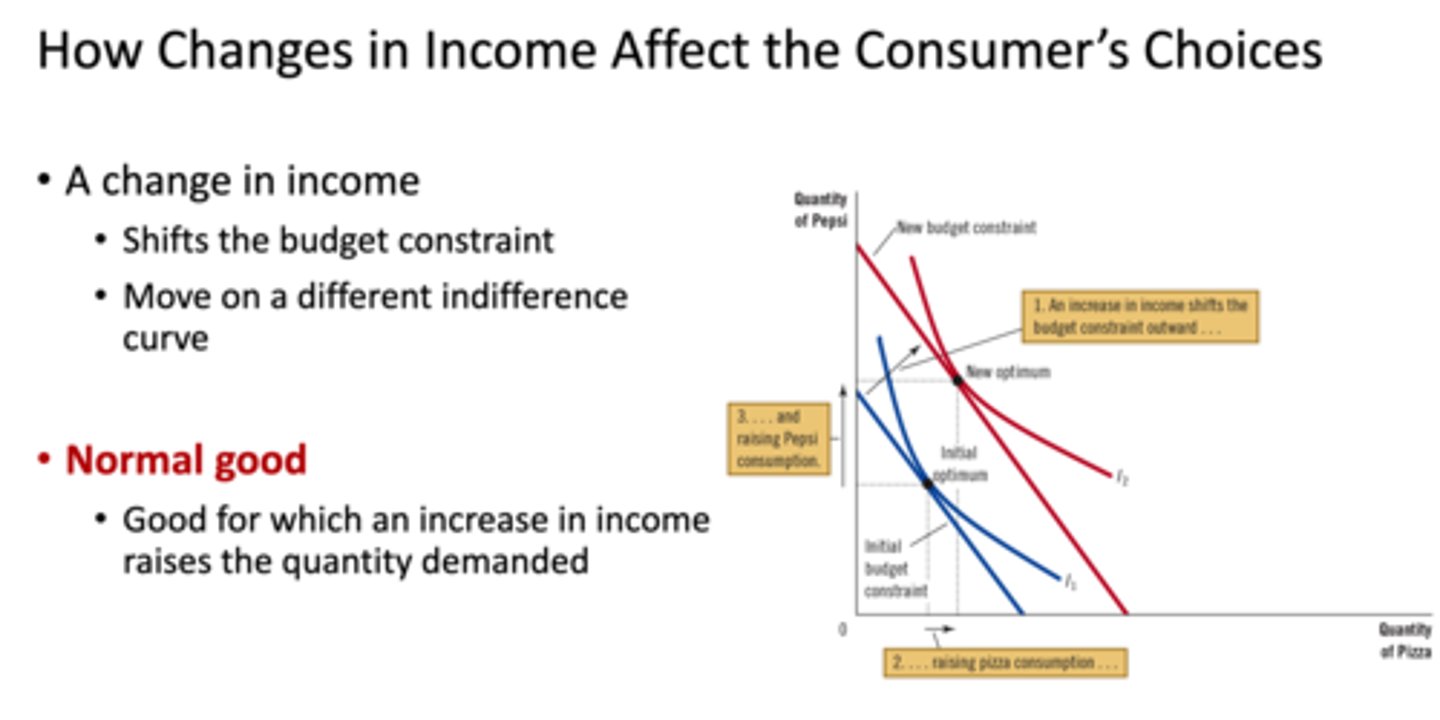
How Changes in Income Affect the Consumer's Choices

Shifts the budget constraint

Move on a different indifference curve

How Changes in Income Affect the Consumer's Choices(Inferior Good)

Good for which an increase in income reduces the quantity demanded

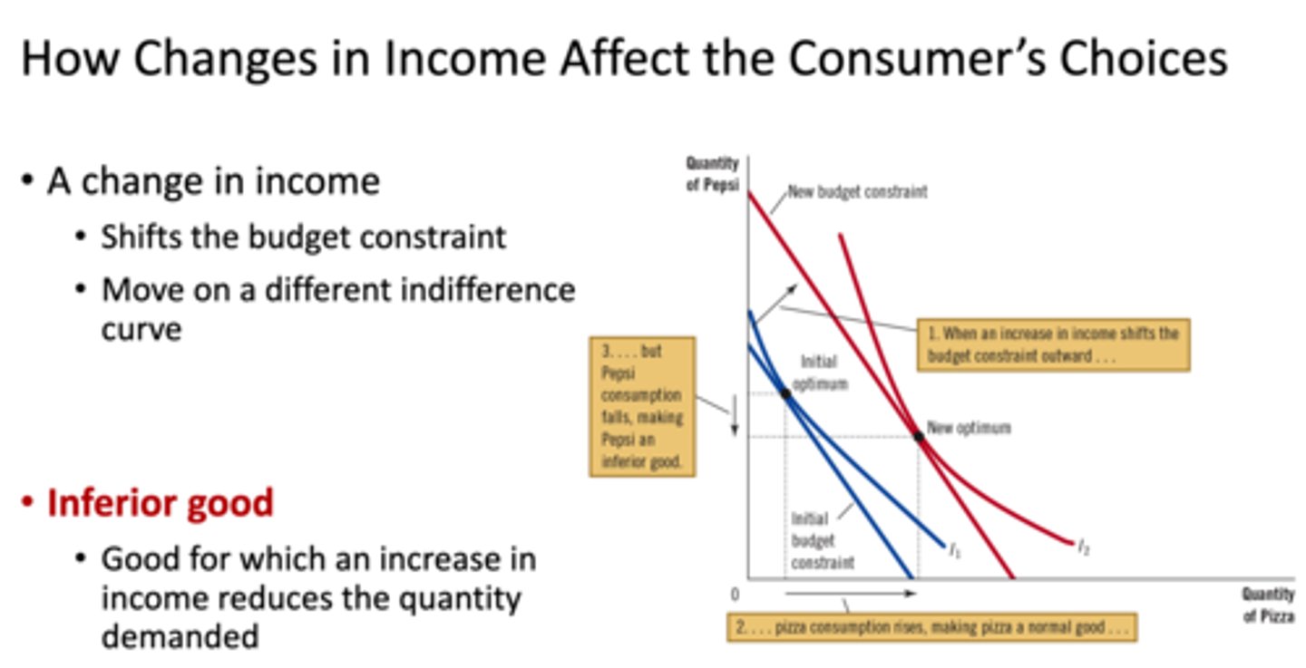
How Changes in Income Affect the Consumer's Choices(Normal Good)

Good for which an increase in income raises the quantity demanded

The Consumer's Optimum

the slope of the indifference curve is equal to the slope of the budget constraint(point where ID Curve and BC meet)

Perfect Substitutes

When two goods are perfectly substitutable, such as nickels and dimes, the indifference curves are straight lines, as shown in panel (a).

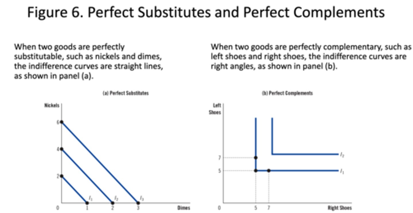
Perfect Complements

When two goods are perfectly complementary, such as left shoes and right shoes, the indifference curves are right angles, as shown in panel (b).

The Consumer's Preferences(Marginal rate of substitution)

The rate at which a consumer is willing to trade one good for another

• Slope of the indifference curve

• Varies along an indifference curve

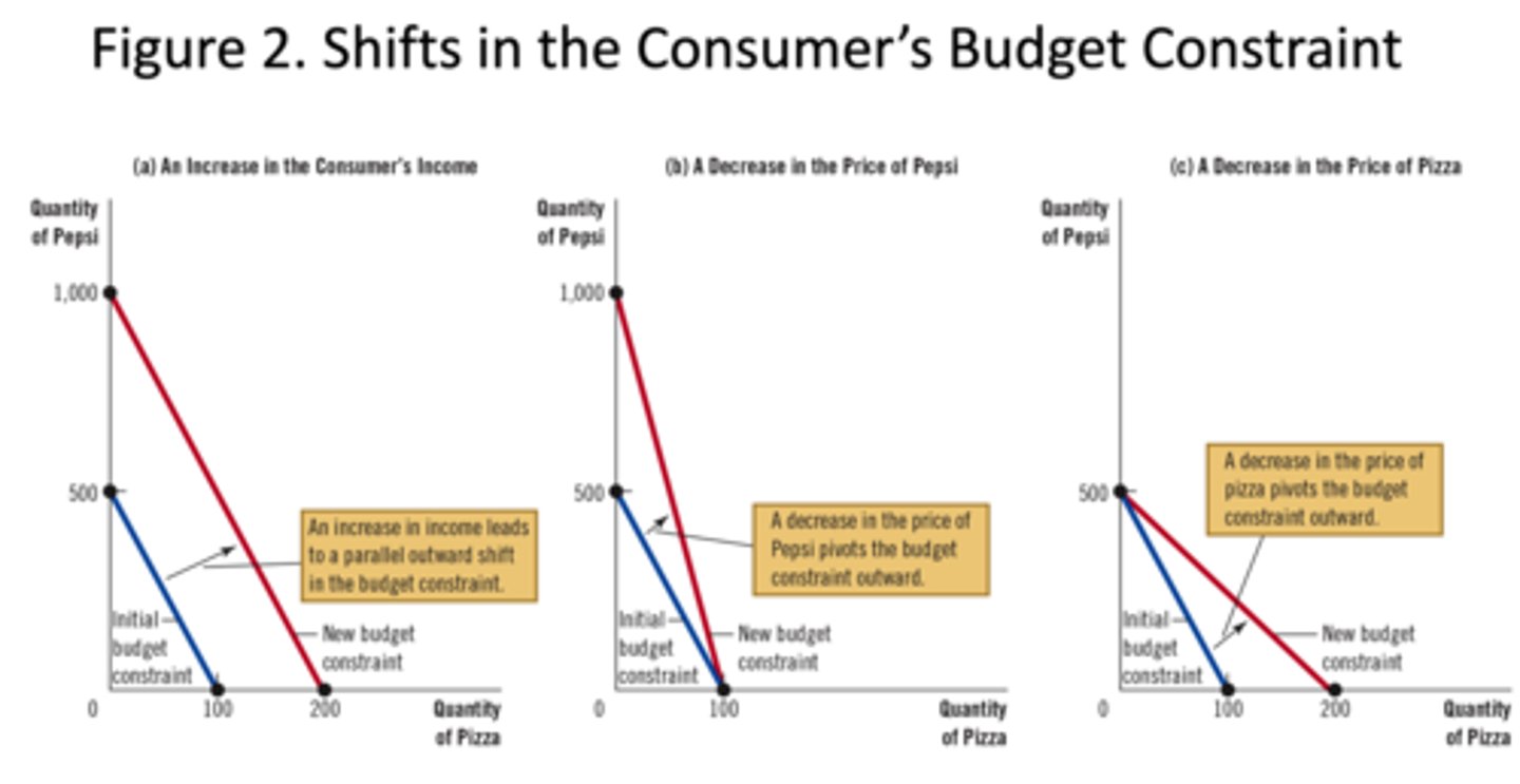
Shifts in the Consumer's Budget Constraint((a) An Increase in the Consumer's Income)

An increase in income leads to a parallel outward shift in the budget constraint.

Shifts in the Consumer's Budget Constraint(A Decrease in the Price of good_y)

A decrease in the price of good_y pivots the budget constraint outward.

Shifts in the Consumer's Budget Constraint(A Decrease in the Price of good_x)

A decrease in the price of good_x pivots the budget constraint outward.

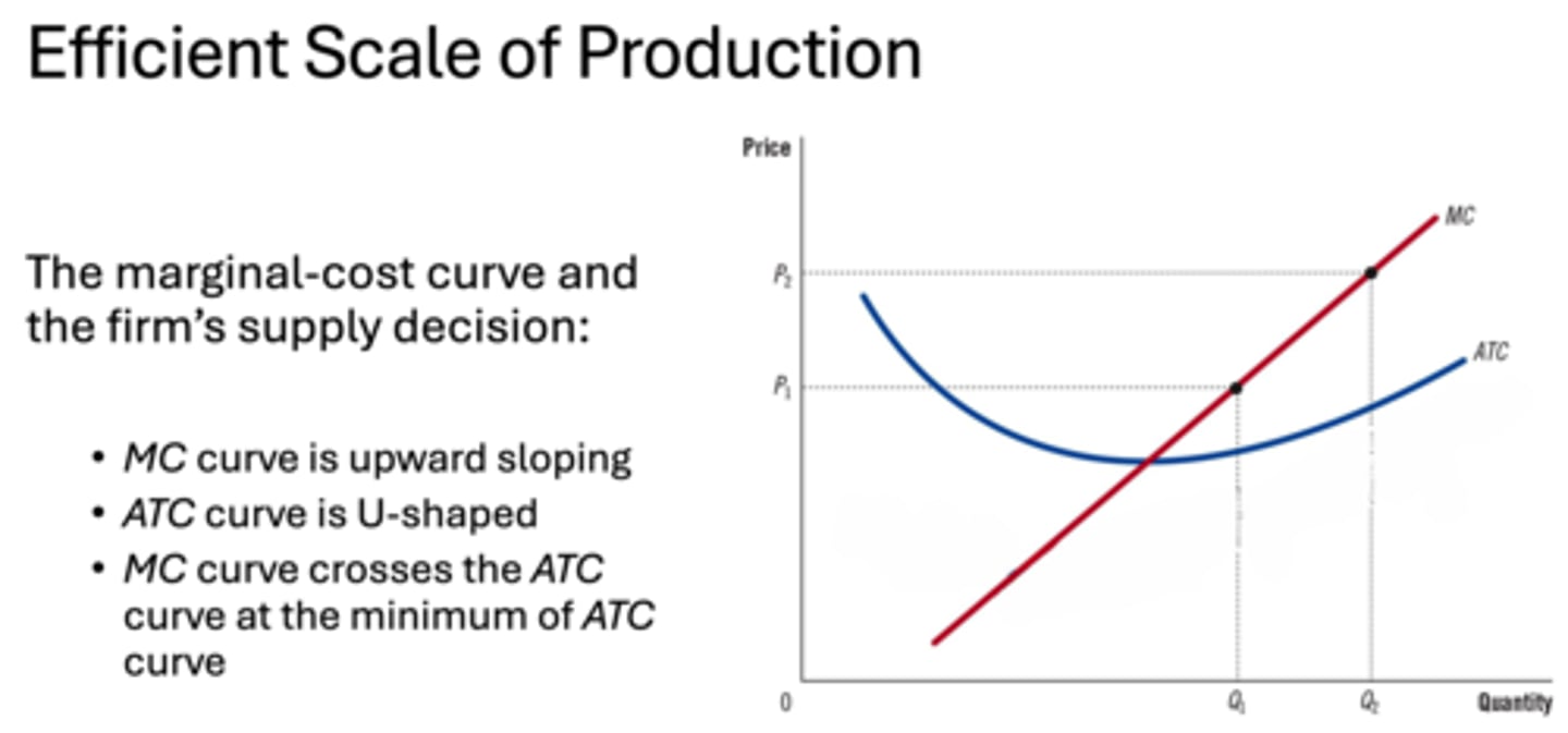
Efficient Scale of Production(The marginal-cost curve and the firm's supply decision)

MC curve is upward sloping

ATC curve is U-shaped

MC curve crosses the ATC curve at the minimum of ATCcurve

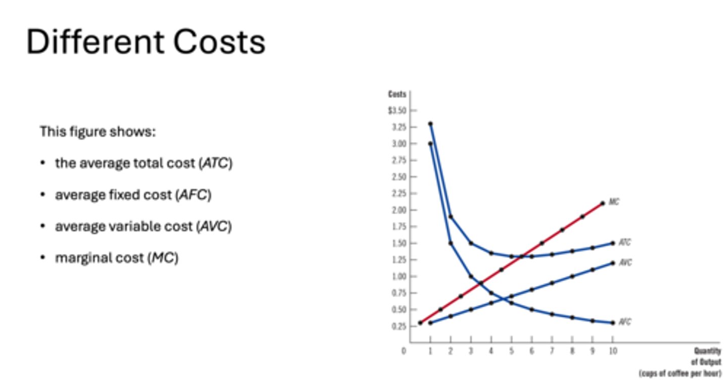
Different Costs

the average total cost (ATC)

average fixed cost (AFC)

average variable cost (AVC)

marginal cost (MC)

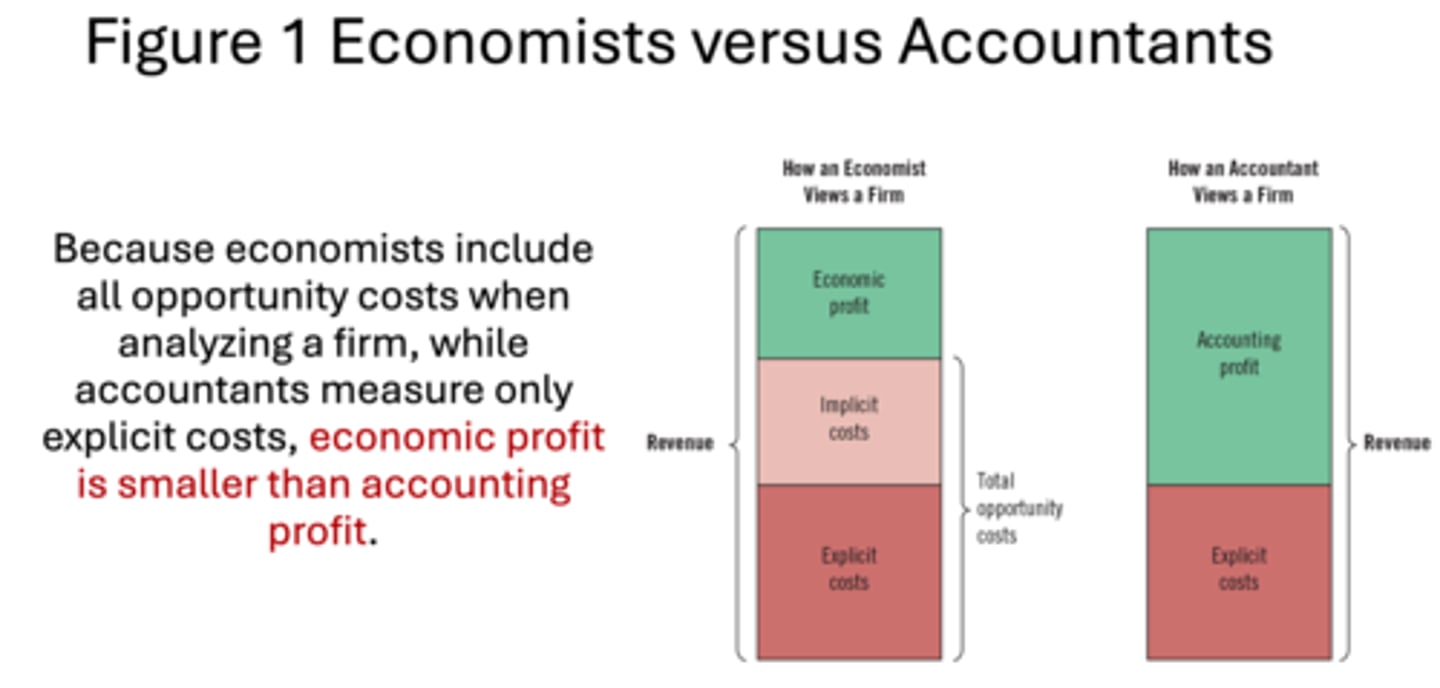
Economists versus Accountants

Because economists include all opportunity costs when analyzing a firm, while accountants measure only explicit costs, economic profit is smaller than accounting profit.

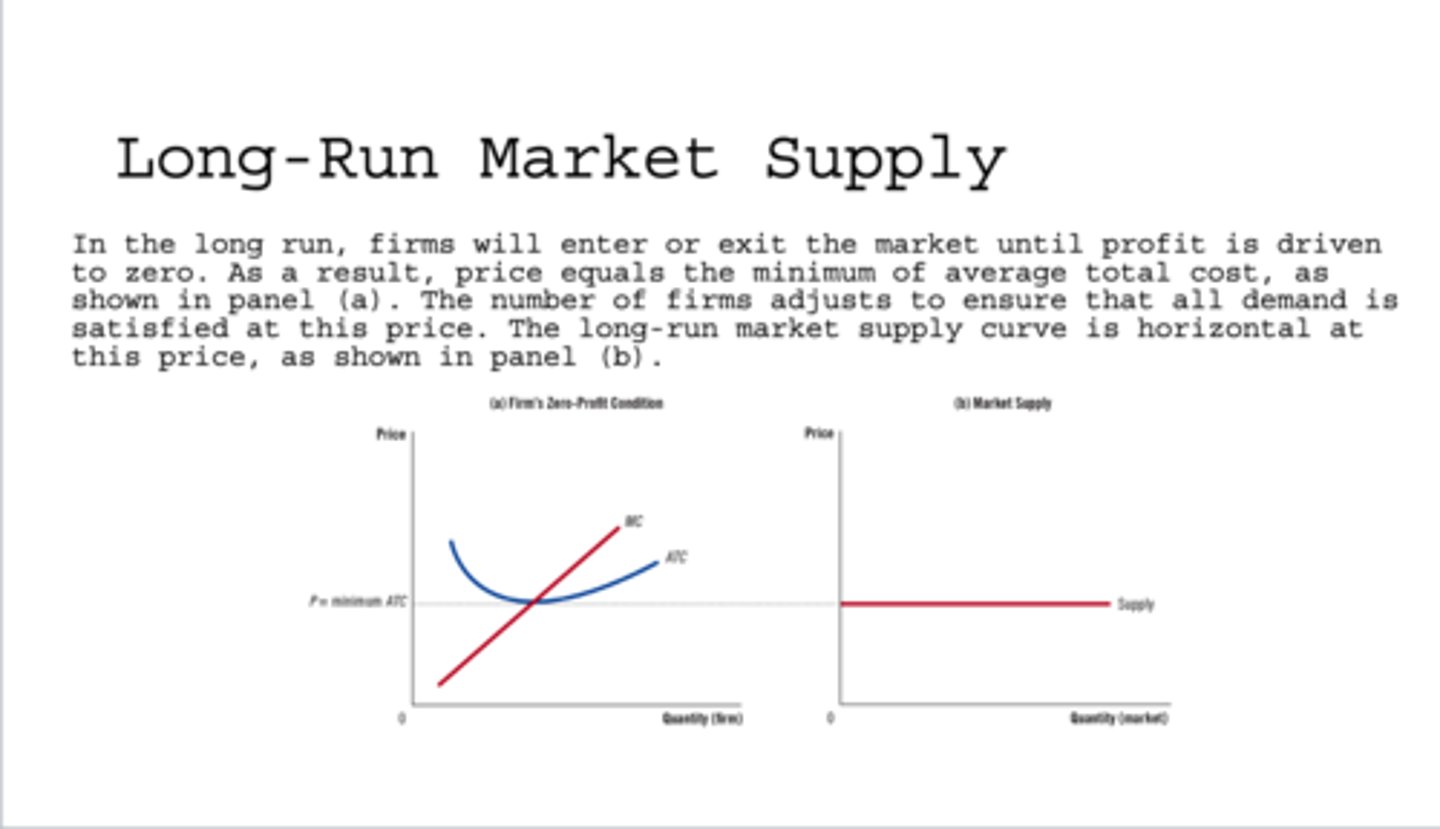
Long-Run Market Supply

In the long run, firms will enter or exit the market until profit is driven to zero. As a result, price equals the minimum of average total cost, as shown in panel (a). The number of firms adjusts to ensure that all demand is satisfied at this price. The long-run market supply curve is horizontal at this price, as shown in panel (b).

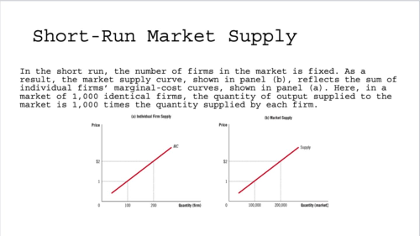
Short-Run Market Supply

In the short run, the number of firms in the market is fixed. As a result, the market supply curve, shown in panel (b), reflects the individual firms' marginal-cost curves, shown in panel (a). Here, in a market of 1,000 identical firms, the quantity of output supplied to the market is 1,000 times the quantity supplied by each firm.

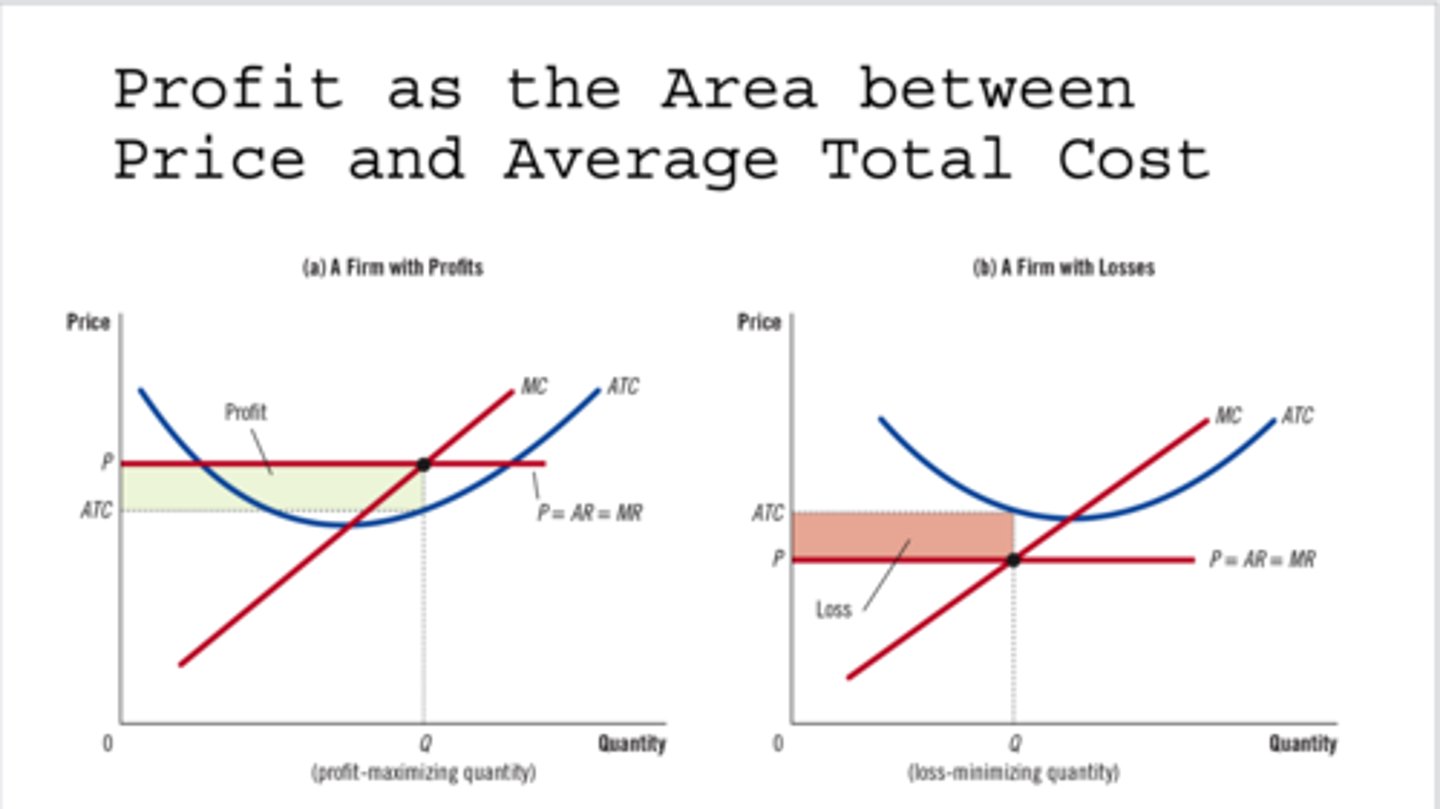
Profit as the Area between Price and Average Total Cost(Profit)

area below Price and above ATC Curve

Profit as the Area between Price and Average Total Cost(Loss)

area above Price and below ATC Curve

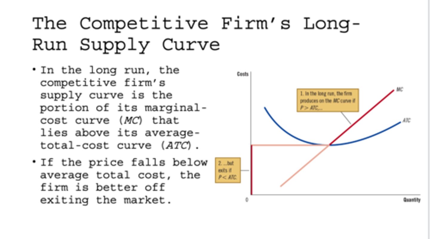
The Competitive Firm's Long-Run Supply Curve

In the long run, the competitive firm's supply curve is the portion of its marginal-cost curve (MC) that lies above its average-total-cost curve (ATC).

• If the price falls below average total cost, the firm is better off exiting the market

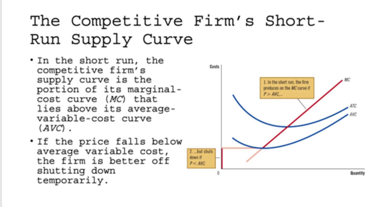
The Competitive Firm's Short-Run Supply Curve

In the short run, the competitive firm's supply curve is the portion of its marginal-cost curve (MC) that lies above its average-variable-cost curve (AVC).

If the price falls below average variable cost, the firm is better off shutting down temporarily.

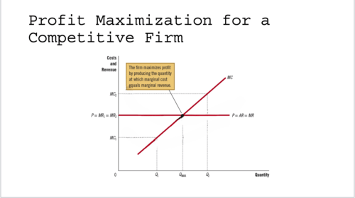
Profit Maximization for a

Competitive Firm

The firm maximizes profit by producing the quantity at which marginal cost equals marginal revenue.

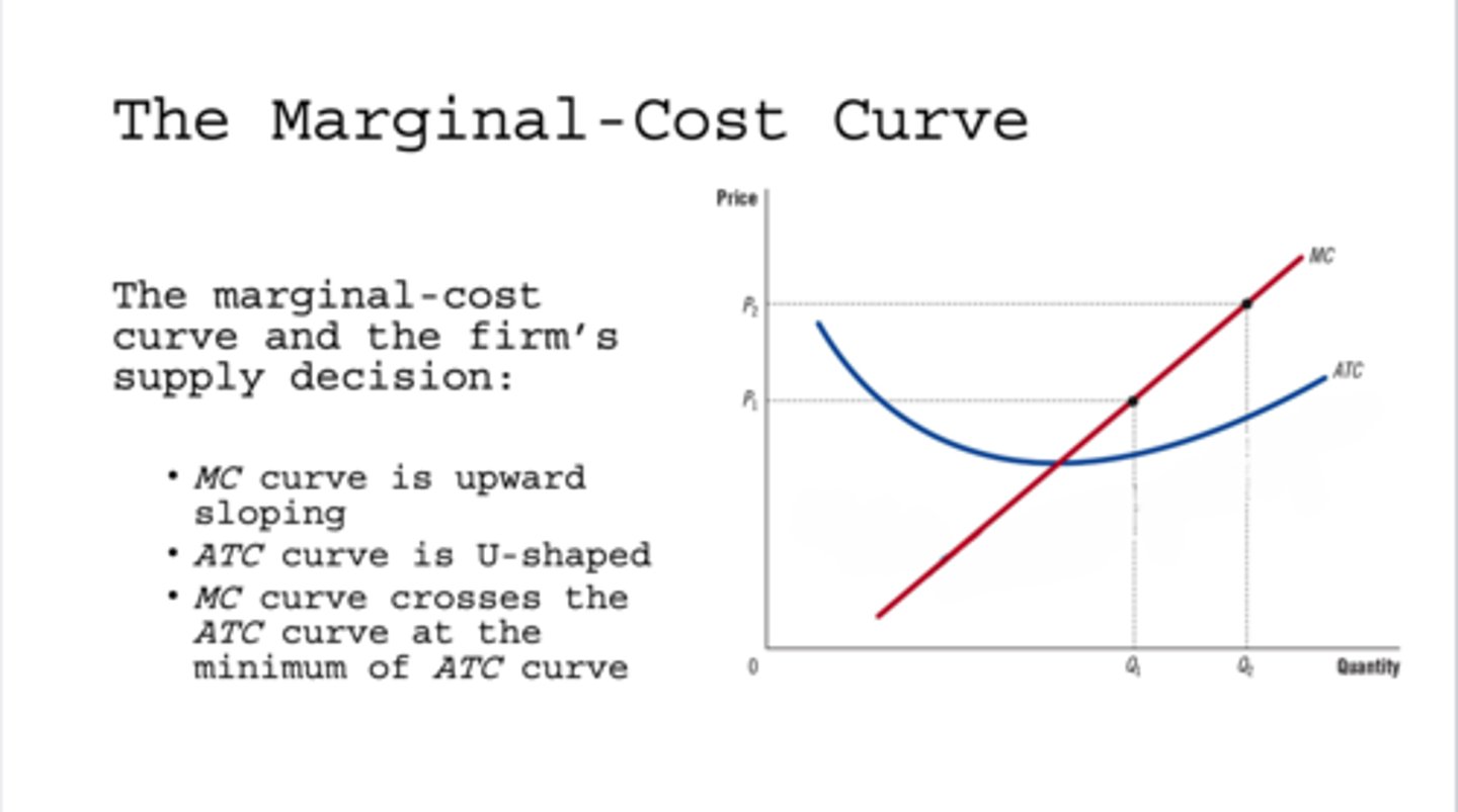
The Marginal-Cost Curve

MC curve is upward sloping

ATC curve is U-shaped

MC curve crosses theATC curve at the minimum of ATC curve

Implicit Cost

Money you could have made, but didn’t—because you chose to use your resources a different way.(input costs that do not require an outlay of money by the firm)

Explicit Cost

input costs that require a direct payment of money by the firm to purchase resources