Stats - linear regression

Population

numerical measurement for a parameter

Sample stats

used to estimate our poluation parameters

Statistical inference

Trying to reach a conclusion (or answer a question) about a complete set of observations (a population) using a subset of observations (the sample)

sample must be representative of pop

3 Features of Statistical inference

• Sample must be representative of pop

• How we make inference → Sampling distributions → Hypothesis Testing

Why do we do hypothesis testing

It helps us make statements about a pop , using a sample of said pop

Hypothesis testing

H0 - hypothesis saying THERES NO STATISTICAL SIGNIFICANCE

HA- is

alpha -sig level - pr of making a type 1 error (false rejection)

test stat- z , t ,

p-val = the pr of getting this test stat ASSUMING THE NULL HYPOTHESIS IS TRUE. If its really low (less than 0.05) we reject H0 , likely that there is some statistical significance

Draw conslusion

Correlation ( what it measures, Pearsons coeff formula, hyp test or r , darwback om cor analysis)

what is measures : Measure of strength + direction of a linear relationship

Calculating pearsons cor coeff : r = SSxy/√SSx√SSy

SSxy = sum ((x-xbar)*(y-ybar))

SSy = sum ((y-ybar)²)

Hyp test to test if r is significant :

1. H0 : p =0

2. HA : p≠ 0

3. T stat → (r√n-2)/√1-r²

(-1 to 1 )

Vs SLR ? → cant predict Y

→ cant forceast effect changing 1 var will have on other

Population vs sample correlation

P - pop cor (direction + strenght of association btwn complete set of variables

r - estimate of p we get from sample

Thresholds for no,low,moderate and high corelation?

0

0.1 to 0.4

0.4 to 0.6

0.6+

Testing if our plotted model (model we made) is significant (good estimate)- R²

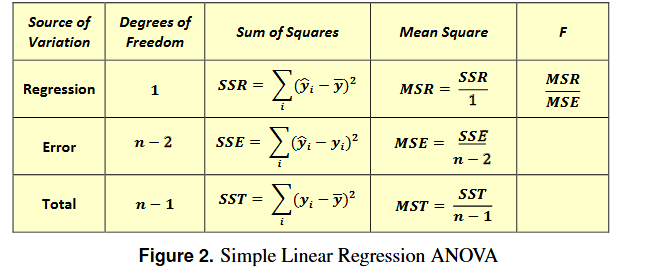
R² ( Coefficient of determination ) → how much var in Y explained by my model

R² = SSr/SSt

Limitations of cor ananlysis

Cant say what impact changing one variable will have on other and cant use it to predict

(only says strenght of relationship and if its likely real or by chance (H0))

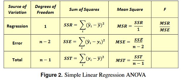
IMPORTANT TO MEMORISE THIS

More SST is made up of SSR means most var in Y captured + explained by our model (good) - model doing good job capturing var in Y

Sample lm and Pop lm equations

• X & Y → continous var

P: Y = b0 (incercept / c) + b1(regression coefficient) x + ei (error term - any var in y thats not becz of x; not all data pts will lie on fitted line exactly)

S : ^Y = ^b0+ ^b1xi

ei= yi^ - yi

why theres no error term for estimate :assume error is normally dist and expected val is 0

Finding b^ estimates

• OLS Algorithim

• Minimising Sum of squared error terms

• How? - trial and error with different b0 and b1 values that give us the smallest squared error - the results are the most optimal estimates )

b coefficients interpretations

• b^0 : avg estimated value of y when x=0

• b^1 : avg estimated increase/decrease of y per unit increase in x

Check for Model accuracy

To measure how acc our linear model is - looks @ std dev of model residuals /how much response deviate from regression line on avg)

closer tg and more on line pts , more accurate our model is

Checking significance of (beta^ parameter)- Se method , calc test stat by hand, in R output)

1. in formula sheet se(B^1) = RSE/√SSx → Interpretation → high se relative to size of estimate (number/magitude of value) = NOT good estimate

• smaller se(shows how diff sample estimate prolly is from pop estimate) , better

• a big se relative to b estimate is fine , when they dont go tg its not

2. Tstat →in formula sheet β^1/se( β^1)) ~ t_n-2

P-val In R → 2* pt (q = test stat , df = , lower.tail = F/T)

Hypothesis test on beta parameters to see if there actaully is a relationship between the variables in the population

Gen goal of Hyp testing → draw conclusions about a pop parameter using the info from a sample of data

confidenece intervals interpretation

95%: if we resample our population we expect 95% of the estimates to be withtin that interval

1. By hand → in formula sheet

Testing overall model significance - RSE, Hyp test w Fstat & R² method

1. RSE plotted - std dev of model residuals ie how much responses deviate from lm line

Lower the better

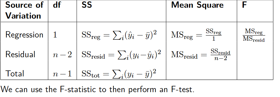
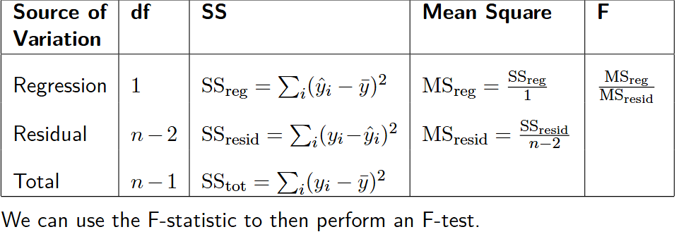
2. check if its significantly different to a null model(model w only a c ) using F stat (bottom row in summary)

H0: B1 = 0

H1: B1 = 0

Fstat =MSreg/MSresid ~ F _n-2

Ftest using Fstat

RSE = √MSresid

2. R² (coefficient of determination)

• looks how much of var in y is explained by x in our model

• 0 - poor model fit , 1 - good model fit

• R² = SSr/SSt

4 linear Model assumptions

1. Relationship btwn X& Y is LINEAR → check w scatter plot

2. E ~ N(0, sigma² )

Errors are….Normal dist w mean = 0 → Histogram : want peak around 0

Constant variance

3. Model errors Independent (no typa pattern going on) →

how do we check linearity

make a scatter plot and look

whats residuals,errors, and residual starndard errors

errors - and variation in why thats not because of /explained by x

residuals - and var in y thats not explained by our model

residual standard error - the standard deviation of the model residuals

Testing if our residuals are normal dist

1. Norm QQ- plot Sample quantities on Y , Theoretical quantities on X

Pts must stick along the red line , normal to have deviation in the tails

2. Histogram (Residulas (x), frequency (y)): Must be bell shaped + centred/peak at 0

Testing our errors : Constant variance and INDEPENDENT

1. Scatter plot of Fitted values (predicted ys from our model) , Residuals ) - Constant var assumption met if even spread of pts around line

2. Scatter plot - (independent variable, residuals)- independent if NO pattern

Prediction - Predicting a Y val in R

• In R → New data.frame where x = …

Predict(model (our lm), newdata= new var where data.frame stored),interval = “prediction”)

• after model checks

• cant predict for x’s outside outside range give

Confience int and Prediction ints cuz our predictions r just estimates

• conf int for the average value of y for a given x

• Prediction intt of the y value for a specific person given their x value

• Conf int for average narrower (smaller) than PI for a certain person cuz more uncertainty in predicting

R studio slr steps

1. maybe read.csv/ read_excel

2. Scatter plot to test linear assumption → plot(x,y)

3. Variance of vars → var(dataset$variable)

4. Std dev of variables → sd(dataset$variable)

5. Cor analysis → cor.test(Y (dataset$…), X (dataset$…))

6. SLR → lm(y ~ x , data = dataset)

7. Plot()

8. Summary()

9. Anova() - this the anova table

10. Confint(), predictionint()