Stats - Writing

Categorical, numerical

What are the two types of variable?

Categorical nominal

Type of qualitative variable in which there is no ranking

Can not be expressed as a number and can not be measured. Names without an order.

categorical ordinal

Type of qualitative variable in which there is an order. Take on numerical values and represent the order of categories. They lack mathematical meaning as spacing between categories not necessarily qual.

Numerical discrete

Type of quantitative variable in which there is a set of values which is specific (no halfs)

Numerical continuous

Type of quantitative variable in which all values are included an in an interval All values in an interval are acceptable

Numerical interval

Type of quantitative data in which its categories are ordered or structural and their spacing is EQUIDISTANT
5+ categories and can be assumed to be equidistant

frequencies, percentages

Data used to describe qualitative data

median, min and max

Data used to describe skewed quantitative data

mean, standard deviation

data used to describe normally distributed data

Variance

Tell us how far from the mean value the values are.

standard deviation

is how spread out a group of numbers is from the mean.

negatively skewed

positively skewed

Random error (noise, random)

Is is a type of error which is unpredictable. Goes on either direction. Either your measurement one time emerges randomly to be higher and another time lower) Due to unknown factors.

systematic error (bias)

Type of error; CONSISTANT. You repeatedly underestimate or overestimate the true values (always in the same direction: one or the other) Due to factors that can be traced in the experimental design (ej. wrong sample, malfunctioning scale, etc)

Sampling distribution

the distribution of a set of estimated means from different samples of the same population

Central Limit Theorem

The theory that, as sample size increases, the distribution of sample means of size n, randomly selected, approaches a normal distribution.
The larger the number off samples the clsoer to the normal distribution

Standard error

the standard deviation of a sampling distribution. How much a sample stat, is likely to vary for the actual population parameter.

The smaller the variability in our population the smaller this measure is (greater precision)
The larger the sample size, the smaller this measure (greater precision)

Hypothesis

A testable statement which entail sour beliefs about observations.

Null hypothesis

Hypothesis that states that something is equal to zero and there is no finding.

We can not accept it; do not have enough evidence to reject it.

Alternative hypotehsis

Hypothesis that states there is a statistical difference, correlation, association, etc.

We can not reject it; not enough evidence to accept it.

Type 1 error

false positive: we think we found significancy but turn out to be wrong

type 2 error

false negative; test incorrectly concludes there is not effect/difference when one truly exists.

power, level of significance, effect size, sample size

What is the group of 4?

Power

Part of the group of 4; we use it to know the sufficient sample size for research. Ability to find the difference if it is actually there.
Type II error; By convention set to 0.8 If there is a difference in the population I am at least 80% confident that I would be able to reveal it.

level of significance

Part of the group of 4; the probability of making a type I error.

Effect size

Part of the group of 4; The size of the effect to be traced; small or large difference, correlation or association.

sample size (n)

how much sample we need to have

A priori power analysis

Before conducting our experiment we compute the SAMPLE SIZE needed to have at least 80% power to detect a difference, with error margin of 0.05. We estimate the effect size based on previous knowledge.

Sample size

What do you calculate on an a priori power analysis

A posterior power analysis

after conducting our experiment we can compute the POWER we actually had to detect a difference, with error margin of 0.05, and the sample size and effect size we actually had.

power

What do you calculate on an a posterior power analysis?

p-value

Is the probability of observing the value we observe, or something more extreme, under the null hypothesis.
Not the probability of being correct.
The smaller this value, the smaller the probability of being wrong.

One sample t-test

Used to determine if a single sample mean is equal to a certain population mean.
Continuous

Assumptions:

Observations are randomly and independently drawn

Symmetrical, bell shaped data

There are no outliers.

Independent samples t-test

Used to test according to the current data, the mean in the population across two groups.

Assumptions:
observations are randomly and independently drawn
symmetrical, bell-shaped data within each group
there are no outliers

continuous data / equality of means

Paired sample t-test

Used to test if, according to the current data, the mean in the population differs across matched groups. (ej. weight before and after).
assumptions:
The (paired) observations are randomly and independently drawn.
the (paired) difference are is symmetrical continuous variable.
There are no outliers in the difference.

continuous data / equality of means

assumptions of independent samples t-test

data are independently sampled
from a normally distributed population
variance of the two groups is the same in the population

Wilcoxon Signed Rank Test

Non parametric test used when the continuous data is skewed in one sample t-test.

Analyze → non parametric → one sample

Assumptions;

The observations re randomly and independently drawn.

At least interval data.

Mann-Whitney U Test (Wilcoxon sum rank)

Used for skewed continuous data in with independent groups.

Assumptions:

• The observations are randomly and independently drawn.

• At least interval data.

Wilcoxon Mathced-Paired Signed Rank test

Used for skewed continuous data in paired groups.

Assumptions:

The pairs of observations ar randomly and independently drawn.

At least interval data

The samples need to dependent observations of the cases. (paired or matched)

One Sample chi-square test

Used to test if according to current data, the proportion, the proportion in the population equals a certain, pre-specified value.

CATEGORICAL data / Legacy dialogs

the observations re randomly and independently drawn.

The number of cells with expected frequencies less than 5, are less than 20%.

The minimum expected frequency is at the the very least 1.

Pearson’s chi-square test

Used to test if, according to the current data, the proportion of 1 variable change based on another variable.

CATEGORICAL data / Crosstabs

In the population, is the proportion of group A equal to the proportion of group B?

Add by column, interpret by row

Add by row, interpret by column (check the one that doesn’t add up to 100)

Assumptions:

The observations are randomly and independently drawn.

The number of cells with expected frequencies less than 5, are less than 20%

The minimum expected frequency is at the very least 1.

The observations are not paired

McNemar Chi-square test

Used to test if, according to the current data, proportions in the population of a variable change based on another matched variable.

CATEGORICAL data / Crosstabs

In the population, is the proportion of a. group in one condition equal to the proportion of the same (or paired) group in another condition?

Assumption:

The observations are randomly and independently drawn.

There are at least 25 observations in the discordant cells.

The data are paired.

discordant cells (yes - no)

What do we base ourselves when checking McNemar test

One sample binomial test

Used when the assumptions fo the one sample chi-square test do not hold.

Categorical data

Fisher’s Exact Test

Used when the assumptions for the Pearson’s chi-square test do not hold

McNemar-Bowker test

usen when the assumptions for the McNemar test are not met…

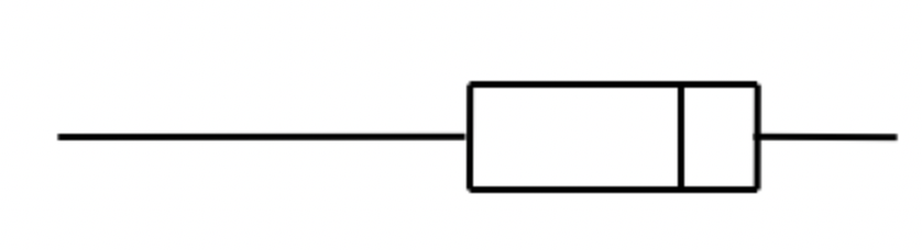
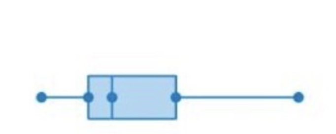
Scatterplots

Used when both the predictor and the outcome are continuous.
The plot of data points x and y with x and y being continuous. It is method for displaying a relationship between 2 variables observed over a number of instances.

Used to investigate an empirical relationship between x (independent) and y (dependent).

correlation

What is r?

correlation ( r)

It represents the strength of the linear relationship

Pearson’s Correlation Coefficient

Used to check magnitude and direction

Assumptiosn:
variables should aproxximately be normally distributed

each variable should be continuous

each participant or observation should have ap air of value

no significant outliers in either variable

linearity, a “straight line” relationship between the variable should be formed.

Spearman’s correlation Coefficient

When one or both of the variables are not normally distributed. This concept of correlation is less sensitive to extreme influential points, so it should be used in the case of non normality.

Used when the data in both variables are skewed (nonparametric version)

Measures the strength and direction of the monotonic relationship between 2 variables

Monotonic relationship

When one variable increases/decreases the other also decreases/increases, but not necessarily at a constant rate, as it does a linear relationship.

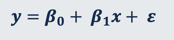
Simple Linear Regression Model

A set of statistical processes for estimating the relationship among variables. It describes the relationship between variables by fitting a line to the observed data.

x

independent variable; predictor/explanantory or covariate variable
Can be continuous or categorical

y

dependent variable, outcome/response; “depends on…”

always continuous

intercept

β₀
value of your takes when x is zero.
If the ______ is zero than y increases in proportion to x (ej. x doubles then y doubles)

predicted value of the dependent variable (y) when x=0

slope (steepness/gradient)

β1 (ONLY for simple linear regression )

Determines the change in y when x changes by 1 unit.

It’s the amount that the dependent that the dependent variable will increase (or decrease) for each unit in the independent variable.

partial regression coefficients

βi’s (β1, β2, β3)

Represent the change in average y for one unite change in x (holding/ adjusting for) all other x’s fixed.

Residual

e

Difference between an observed value and a value predicted by a stats model. Distance between points and the line of best fit.

The best linear regression line is the one closes to all data point - makes this variables as small as possible.

ordinary least square

method used to find the best‑fitting straight line through your data.
Is one method that can be used to estimate the regression line that

minimises the squared residuals to give us the estimates for 𝜷𝟎 and𝜷𝟏.

Simple Linear Regression Model

Used to measure to what extent there is a linear relationship between 2 variables.

Ho = there is no linear association (𝜷𝟏. = 0)

Ha: There is a linear association (𝜷𝟏 not equal 0)

Assumptions:

There is a linear relationship between the dependent and independent variable

• Residuals (or “errors”) ε are independent of one another: the observations in the dataset were collected using statistically valid sampling methods, and there are no hidden relationships among observations

• Residuals follow a Normal distribution, with mean 0 and constant Standard Deviation σ

• Homogeneity of variance (homoscedasticity): the size of the error in our prediction doesn’t change significantly across the values of the independent variable.

Homoscedasticity

When scatter plot seemed to follow a general linear pattern

r value

value of strength for a simple correlation

r squared value

indicates how much of the total variation in the dependent value, y, can be explained by the independent value, x.

ej. 27% of weight can be explained by height.

Association studies:
how much of the variation in y is explained by x

Prediction context:

How well does the model predict your values from x

does not indicate:

whether the independent variables are a cause of the changes in the dependent variable; we can only say they are associated.

the correct type of association was used

most appropriate set of independent variables have been chosen

there are enough ata points to make a solid conclusion

ANOVA

reports how well the regression equation fits the data. We interpret its p-value.

Multiple Linear Regression model

Allows us to hold all other variables constant, allowing us to get an estimate of the effect of the independent variable of interest, while adjusting for other variables in the model which are hypothesized confounders.

There are multiple explanatory variables. Can deal with multiple confounders (within reason)

Use it as a method to study the relationship between 1 dependent variable (ej. weight) and 2+ independent variables simultaneously (ej. exercise, diet, etc.) to understand how a dependent variable can be explained by a set of other variables.

Ho = holding all other variables constant, there is no linear association between y and x1

holding all other variables constant, there is linear association between y and x1

Aim to answer:

whether and how several facts are related with one other fact?

whether and how a set of independent variables are relates with a dependent variables.

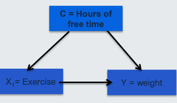
confounder

A situation in which the association between an explanatory variable (e.g exercise 𝒙𝟏) and outcome (e.g. weight y) is distorted by the presence of another variable (e.g. hours of free time 𝐱𝟐).

This variable has a common effect on the independent and dependent variables. Is extrinsic (not part of) to the causal pathway.

confounding varialbes

any other variable that cause both your dependent and your main independent variable of interest. It’s like a “extra independent variable” having a hidden effect on your dependent variables, while being related to the independent variable of interest.

If not taken into account, will introduce bias in the estimation of β1.djA

Adjusted R squared

is modified version the adjusts for the number of independent variables in the model. The other one increases every time an extra independent variable is added regardless of whether it has an effect or not.

This one increases only when the new variable actually improves the model more than you’d expect by chance.

Assumptions for Multiple Regression Inference

1. The relationship between the dependent (y) and each continuous independent variable (x variables) is linear.
   How to check:

   • Scatter plots of Y vs each X variable.

2. Residuals (error terms) e should be approximately normally distributed

3. Homoscedasticity - stability in variance of residuals

4. Independent observations

ZRESID

when testing for assumptions to make inference from a multiple linear regression… which one needs to be added to y?

ZPRED

when testing for assumptions to make inference from a multiple linear regression… which one needs to be added to x?

mediator

explains a portion of the association between Y

and x1.

_______ of the causal effect of independent variable (x1) on dependent variable (Y) is a variable x2 on nonthe causal pathway from x1 to Y.

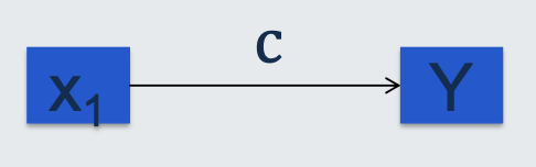
non-mediated model

the total effect of the independent variable x1 on the dependent Y is denoted by the path 𝑐

mediated model

the total causal effect 𝑐 can be split into an indirect (or mediated) part with paths 𝑎 and 𝑏 and a direct (non-mediated) path

c’

It’s the direct non-mediated path between x1 and y

path c

In the mediator model is the total effect of the variable x1 on y (both direct and indirect)

Total effect
Simpel linear regression between x1 and y (tell us how much y changes when x increases by 1)

Y= β0 + β X1+ε

a * b

indirect effect in the mediated model

path a

Simple linear regression between the mediator and the main independent variable

x1 → Mediator

M= β0 + β1X1 +ε

path b

Multiple linear regression that give us value of pathway b

Y = β0 + β2M +β3X1+ε

path c

Step1 of the Baron and Kenny steps test for….

(x1 → y)

Establish that the causal variable x1 is associated with the dependent y

path a

Step 2 of the Baron and Kenny steps test for….

(x1 → M)

Show that the causal variable x1 is associated with the mediator

path b

Step 3 of the Baron and Kenny steps test for….

(M → y, adjusting for x1)

Shows the mediator M is associated with Y, adjusting for the causal variable x1

path c’

Step 4 of the Baron and Kenny steps test for….

(x1 → y, adjusting for M)

complete mediation

No significant association between x1 and y, when we control for M.

B3 is not significatn

partial mediation

There is a significant association between x1 and y, when we control for M.

modifier

is a variable that alters the relationship between the independent X1 and idependent Y variables.

interaction term

the cross-product between x1 and the modifier z

(x1 * z)

outlier

is an observation that lies an abnormal distance from other values in a random sample from a population.

can be problematic for many statistical analyses because they can cause tests to either miss significant findings or distort real results.

generally serve to increase error variance and reduce the power of statistical tests.

Evaluate to remove an outlier

• if it appropriately reflects your target population, subject-area, research question, and research methodology.

• Did anything unusual happen while measuring these observations, such as power failures, abnormal experimental conditions, or anything else out of the norm?

• Is there anything substantially different about an observation, whether it’s a person, item, or transaction?

• Did measurement or data entry errors occur?

to remove or not to remove

A measurement error or data entry error, correct the error if possible. If you can’t fix it, remove that observation because you know it’s incorrect.

Not a part of the population you are studying (i.e., unusual properties or conditions), you can legitimately remove the outlier.

A natural part of the population you are studying, you should not remove it.

Odds

describes the ratio of the number of people with the event to the number without.

relative risk

is the probability of an adverse outcome in an exposure group versus its likelihood in an unexposed group. This statistic indicates whether exposure corresponds to increases, decreases, or no change in the probability of the adverse outcome.

RR equals one

The risk ratio equal 1 when the numerate rand denominator are qual.

exposed group = unexposed group

Equivalence (the probability of the event occurring int he exposure group is equal to the likelihood of it happening in the unexposed group)

ej. There is no association between mothers smoking status and baby being born with a low birth weight.

Equivalence

the probability of the event occurring int he exposure group is equal to the likelihood of it happening in the unexposed group

RR is greater than one

The numerator is greater than the denominator in the risk ratio. Therefore the event’s probability is greater in the exposed group than in the unexposed group (risk value).

Ej. if the RR = 1.4, the smoking status corresponds to a 40% greater probability of a mother having a child with low birthweight.

RR is less than one

The numerator is less than the denominator in the risk ratio. Consequently, the probability of the event is lower in the exposed group than the unexposed group (protective value).

ej. if the RR = 0.4, the smoking state corresponds to a 60% lower probability of another having a child with low birthweight.

OR equals 1

odds of 1 mean the outcome occurs at the same rate in both groups. Exposure doesn’t affect the odds of outcome.

Ej. There is no difference in the odds of low birth rate between smokers and non-smokers.