Artificial Intelligence with Deep Learning

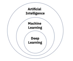
artificial intelligence (AI)

• an umbrella term for computer software that mimics human cognition in order to perform complex tasks and learn from them

Goals of AI

• to understand the principles that make intelligent behaviour possible

• to create expert systems → simulate the decision-making ability of a human expert

• to implement human intelligence in machines

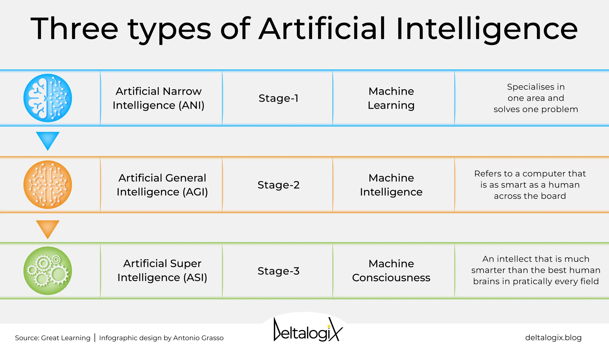
Types of AI

1. Narrow AI (Weak AI):

- systems designed to perform a narrow task (e.g., facial recognition or internet searches)

2. General AI (Strong AI):

- hypothetical systems that possess the ability to perform any intellectual task that a human being can do

3. Superintelligent AI:

- an AI that surpasses the cognitive abilities of humans in all respects

- speculative and largely theoretical at present

Machine Learning (ML)

• a subfield of AI that uses algorithms trained on data to create adaptive models that can perform a variety of complex tasks

Goals:

• automation

• adaptation

• generalization

• interpretability

• scalability

Applications:

• prediction → estimating the output or future values based on input data

• classification → assigning input data to predefined categories or classes

• regression → determining the relationship between variables to predict continuous outcomes

• clustering → grouping similar data points into clusters or groups without predefined labels

• anomaly detection → identifying outliers or unusual patterns in the data

• dimensionality reduction → reducing the number of variables or features in data while retaining its essential characteristics

• reinforcement learning → learning optimal actions through trial and error by maximizing cumulative reward

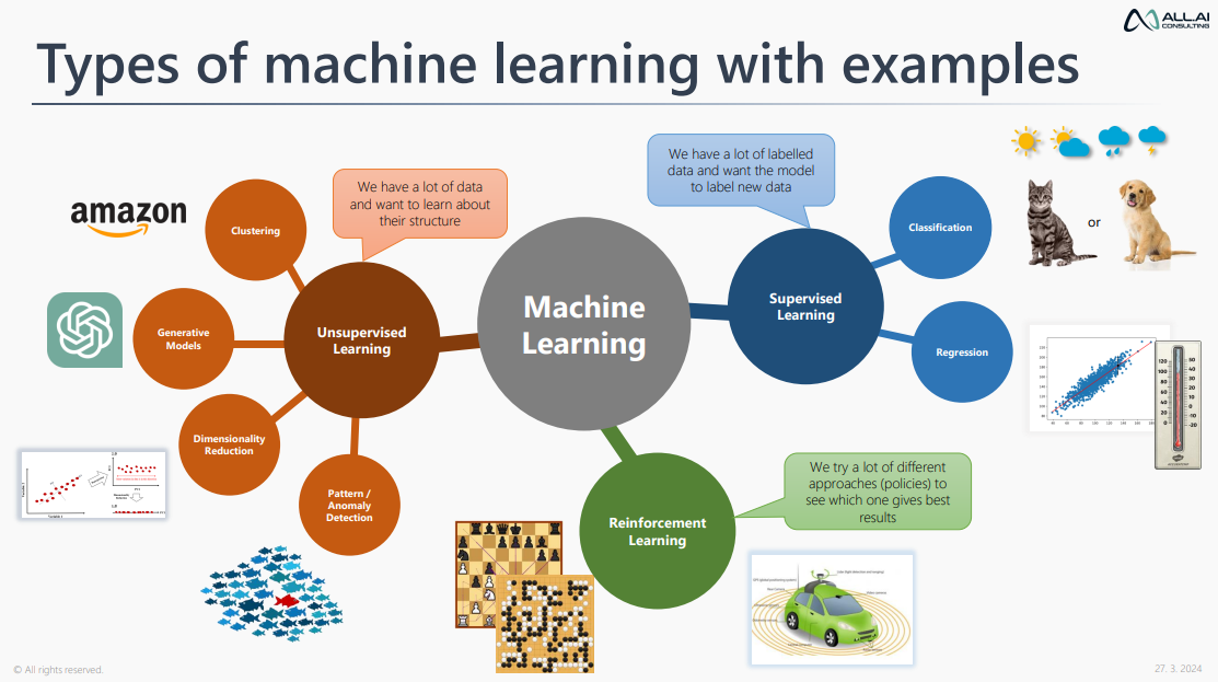
Common ML Techniques & Approaches

1. Supervised Learning → learning from labeled data where the algorithm is trained on input-output pairs.

e.g. training a model to recognize cats and dogs from labeled images

2. Unsupervised Learning → learning from unlabeled data to identify hidden patterns or structures.

e.g. clustering customers based on purchasing behavior

3. Semi-Supervised Learning → combines a small amount of labeled data with a large amount of unlabeled data to improve learning accuracy

4. Reinforcement Learning → learning based on rewards and penalties through interactions with the environment.

e.g. training a robot to navigate a maze

5. Deep Learning → utilizing neural networks with many layers (deep networks) to learn representations and patterns from large datasets

Deep Learning (DL)

a branch of machine learning that uses multiple layers in neural networks to perform some of the most complex ML tasks without human intervention

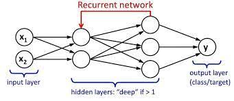
• multilayer/deep artificial neural networks

• inspired by biological nervous systems

• input layer, hidden layers, and output layer interconnected via nodes/neurons

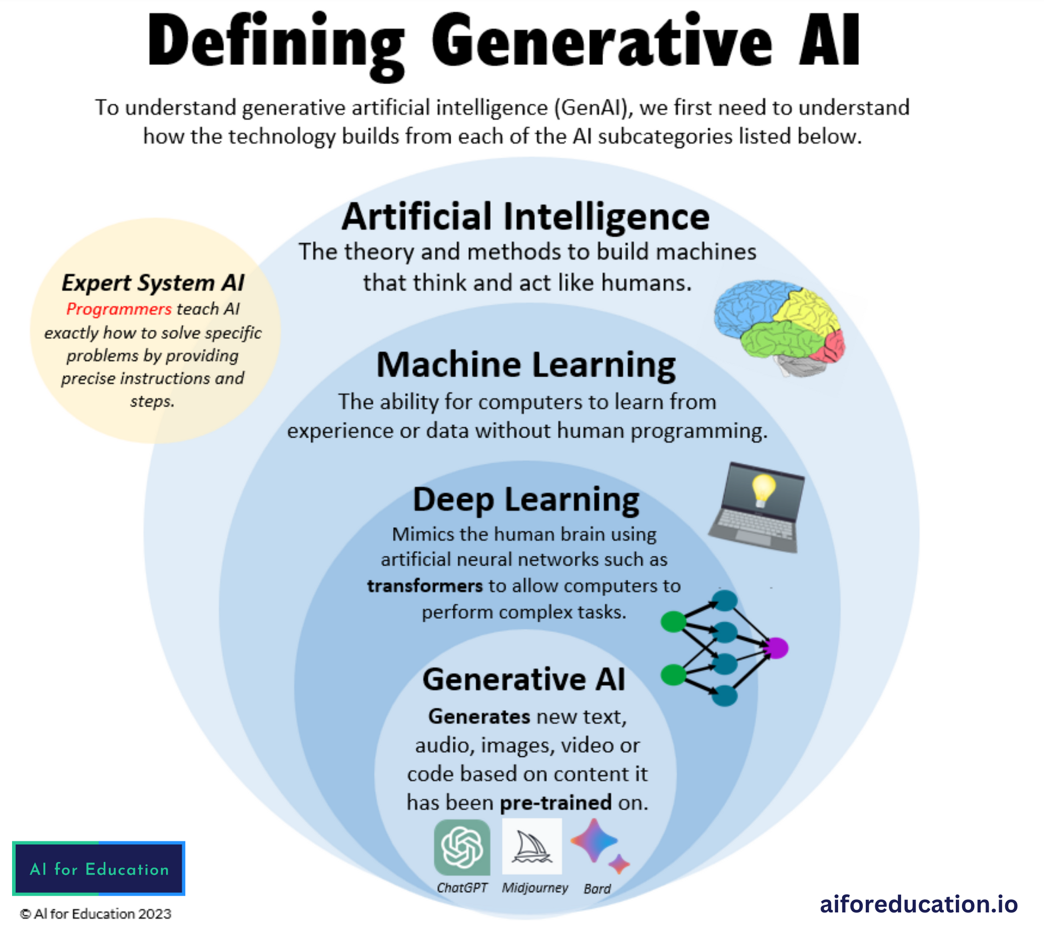
Generative Artificial Intelligence (GAI)

a machine learning approach in which AI models are learned from patterns and structures of input training data to generate new data, text, images, software, or other data formats with similar characteristics to the input data, often in response to prompts

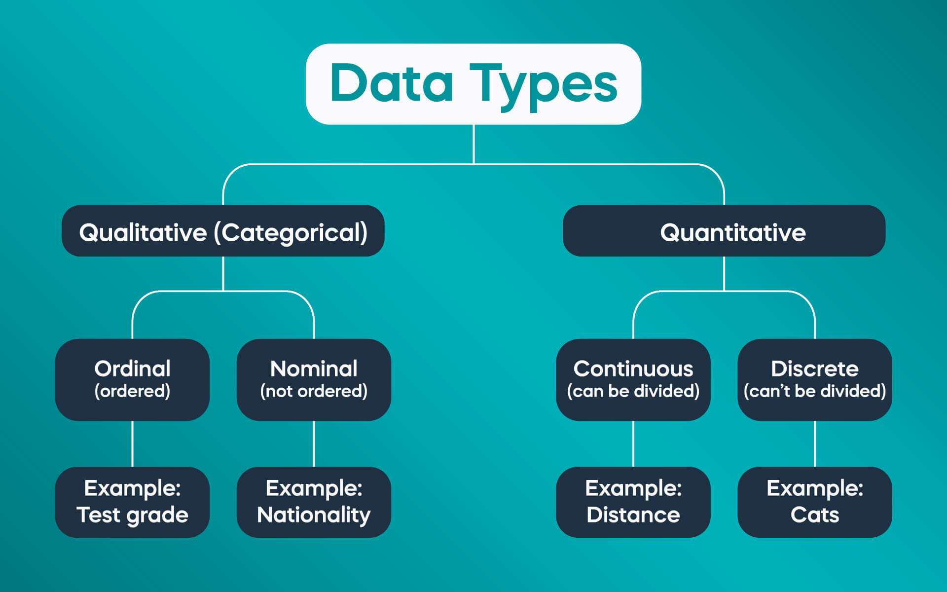
data types

1. Numerical Data:
- represents quantitative information, such as numbers, measurements, or counts
- discrete data → can only take on specific, countable values, such as integers
- continuous data → can take on any value within a given range, such as floats

2. Categorical Data:
- represents qualitative information, such as labels or categories
- nominal data → no inherent order or ranking (e.g. gender, color, country)
- ordinal data → has a specific order or ranking, such as ratings (e.g., low, medium, high) or educational levels

3. Text Data:
- unstructured information, such as natural language text, documents, or transcripts

4. Image Data:
- visual information, such as photographs, illustrations, or diagrams

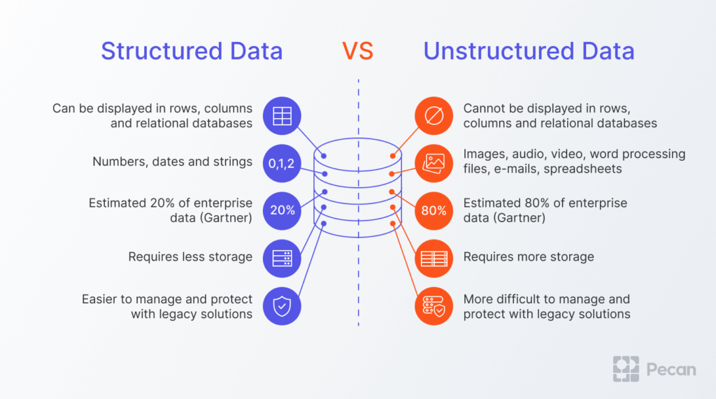
Structured vs Unstructured Data

• structured data is highly organised and formatted in a way so it's easily searchable in relational databases

• unstructured data has no pre-defined format or organization, making it much more difficult to collect, process, and analyze

planning vs scheduling

PLANNING

• determining a sequence of actions to achieve a specific set of goals given the initial conditions and constraints

• devising a strategy to achieve specific objectives

SCHEDULING

• assigning specific time and resources to a set of pre-defined tasks or actions

types of knowledge

1. Declarative Knowledge

2. Procedural Knowledge

3. Tacit Knowledge

4. Explicit Knowledge

5. Common-Sense Knowledge

6. Domain-Specific Knowledge

7. Meta-Knowledge

8. Heuristic Knowledge

9. Structural Knowledge

declarative knowledge

• facts and information about the world that can be directly asserted → can be expressed in words

• easy to communicate

e.g. Paris is the capital of France

procedural knowledge

- knowledge of how to do something, such as riding a bike

- expressed in behaviors rather than in words → difficult to verbalize

tacit vs explicit knowledge

- tacit knowledge is personal and context-specific knowledge that is hard to formalize and communicate → internalized through experience

- explicit knowledge is knowledge that can be easily articulated, documented, and shared → codifiable

Meta-knowledge

- knowledge about knowledge itself, including understanding the structure, usage, and management of knowledge

- self-referential

heuristic knowledge

- rules of thumb related to a problem or discipline derived from experiences and observations

- lead to satisfactory solutions

ontology

• formal representation of a set of concepts within a domain and the relationships between those concepts

• model domain knowledge in a structured way that can be interpreted by machines

• classes → entities or things within the domain

• instances → specific examples of classes

• attributes → characteristics or properties of classes

• relationships → how classes and instances are related

• axioms → rules that define constraints and logical assertions about the classes and relationships

Natural Language Processing (NLP)

- subfield of AI that focuses on interaction between computers and human languages

- goal → enable computers to understand, interpret, generate, and respond to human language in a way that is both meaningful and useful

Applications of NLP:

- sentiment analysis → understanding the sentiment or tone behind a piece of text, widely used in social media monitoring, and customer feedback analysis...

- spam detection

- language translation

- content recommendation

- legal document analysis

ML workflow

1. Project/Problem Definition
- define the problem that you are trying to solve
- determine success metrics to evaluate the model

2. Data Collection
- gather the data necessary to train and evaluate the model

3. Data Preprocessing
- prepare the data for machine learning by cleaning and transforming it
- feature engineering → create new features based on existing data
- split data into training, validation, and test sets

4. Exploratory Data Analysis (EDA)
- understand the underlying patterns and characteristics of the data → visualizations, statistical analysis, outlier detection

5. Model Selection
- choose an appropriate machine learning algorithm or model for the task

6. Model Training
- train the selected model using the training data
- hyperparameter tuning → adjust the hyperparameters of the model to optimize performance
- cross-validation → use cross-validation techniques (e.g. k-fold) to ensure the model generalizes well to unseen data

7. Model Evaluation
- assess the performance of the trained model using validation and test data → performance metrics
- confusion matrics
- ROC/AUC

8. Model Interpretation and Validation
- ensure the model's predictions are understandable and reliable
- feature importance scores
- model explainability

9. Model Deployment
- implement the trained model in a production environment to make real-time predictions
- continuously monitor the model's performance

10. Model Maintenance and Updating
- ensure the model remains accurate and relevant over time
- retraining → periodically retrain the model with new data to keep it updated

Representation/feature learning

- focuses on automatically discovering the representations or features needed for classification, regression, or other tasks from raw data

- transform raw data into a format that makes it easier for ML algorithms to extract useful patterns and make accurate predictions → improving the performance, generalization, and scalability of ML models

- feature extraction → automatically learn features from raw data that are relevant to the task at hand

- dimensionality reduction → reduce the complexity of the data by transforming it into a lower-dimensional space while preserving important information

- invariance and robustness

- data compression → compress data into a compact representation that retains essential information

- generalization → learn features that generalize well to new, unseen data

Reinforcement learning

• a ML technique that trains software to make decisions to achieve the most optimal results

• mimics the trial-and-error learning → learning the optimal behavior in an environment to obtain maximum reward

• agent → the learner or decision-maker that interacts with the environment

• the agent's primary goal is to learn a policy that maximizes the expected cumulative reward over time

• the agent receives feedback from the environment in the form of rewards

• the agent continuously learns and updates its policy based on ongoing interactions with the environment

• value function → quantitative representation of the expected cumulative future rewards an agent can obtain in different states or state-action pairs

Trustworthy AI

- developing artificial intelligence systems that are reliable, ethical, and socially beneficial

- human-centric → should amplify human agency; needs to have a positive social impact

- accountability → companies need to take responsibility for their AI systems (safety, security, resilient, valid, reliable, fair)

- transparency and explainability → must be understandable to the intended audience (technical, legal, end-user)

- fairness → AI systems are free from biases and do not discriminate against individuals or groups

- sustainability → AI systems contribute to sustainable development and do not harm the environment

ML tasks

- nature of the learning signal or feedback available to the system

1. Supervised Learning

2. Unsupervised Learning

3. Semi-supervised Learning

4. Reinforcement Learning

5. Self-supervised Learning

6. Multi-instance Learning

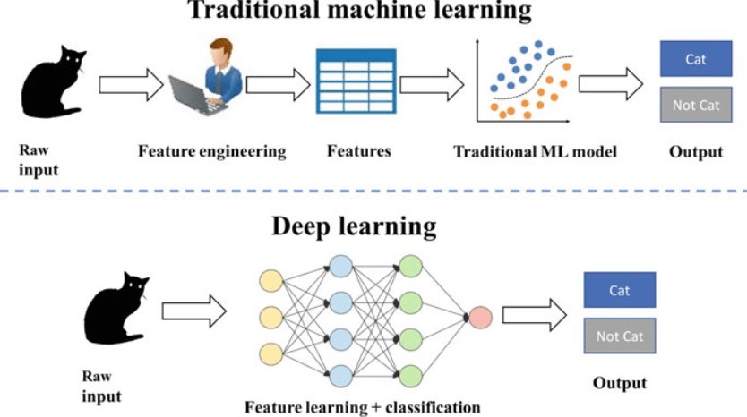
Deep Learning vs Machine Learning

- ML and DL are both types of AI

- machine learning is AI that can automatically adapt with minimal human interference

- deep learning is a subset of machine learning that uses artificial neural networks to mimic the learning process of the human brain

- ML is best for well-defined tasks with structured and labelled data

- Deep learning is best for complex tasks that require machines to make sense of unstructured data

- ML typically requires manual feature engineering, while deep learning solutions perform feature engineering with minimal human intervention

- ML has four main training methods → supervised learning, unsupervised learning, semi-supervised learning, and reinforcement learning

- deep learning algorithms use several types of more complex training methods → convolutional neural networks, recurrent neural networks, generative adversarial networks, and autoencoders

- Deep learning is more complex with a very high data volume

Supervised Learning

- algorithms are trained by providing explicit examples of results sought, like defective versus error-free, or stock price → requires a labelled dataset

- training data consists of one or more inputs and a desired output, also known as a label

- classification → assigning a label to an instance from a discrete set of categories (e.g. spam filtering, disease prediction)

- regression → predicting a continuous continuous value for an instance (e.g. weather forecasting)

e.g. linear regression, decision trees, SVMs, neural networks

Unsupervised Learning

- learning patterns from untagged data → system tries to learn without any explicit instructions

- uncovering hidden patterns or intrinsic structures in input data

- clustering → discovering groups in the data where members of a group are more similar to each other than to those from other groups

- dimensionality reduction → reducing the number of random variables to consider

- association → sets of items or events that often occur together

e.g. K-means clustering, hierarchical clustering

Semi-Supervised Learning

• it uses both labelled and unlabeled data for training

• improve learning accuracy by using large amounts of unlabeled data

• text classification

• image recognition

Binary Classification

- supervised learning algorithm → classifying the elements of a set into one of two groups/classes

e.g. determining whether an email is "spam" or "not spam."

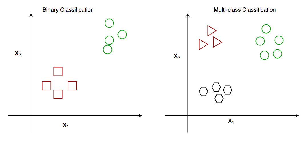
Multi-class Classification

- the process of assigning entities with more than two classes

e.g. classifying an image as either a cat, dog, or horse

Multi-label Classification

- assigning multiple labels to an instance, allowing it to belong to more than one category simultaneously

- the model outputs multiple binary values, one for each label, indicating the presence or absence of each label independently

e.g. tagging a news article with multiple relevant categories such as "politics," "economy," and "environment."

Single-target vs multi-target regression

• single-target regression involves predicting a single continuous value for each input

• multi-target regression involves predicting multiple continuous values simultaneously for each input

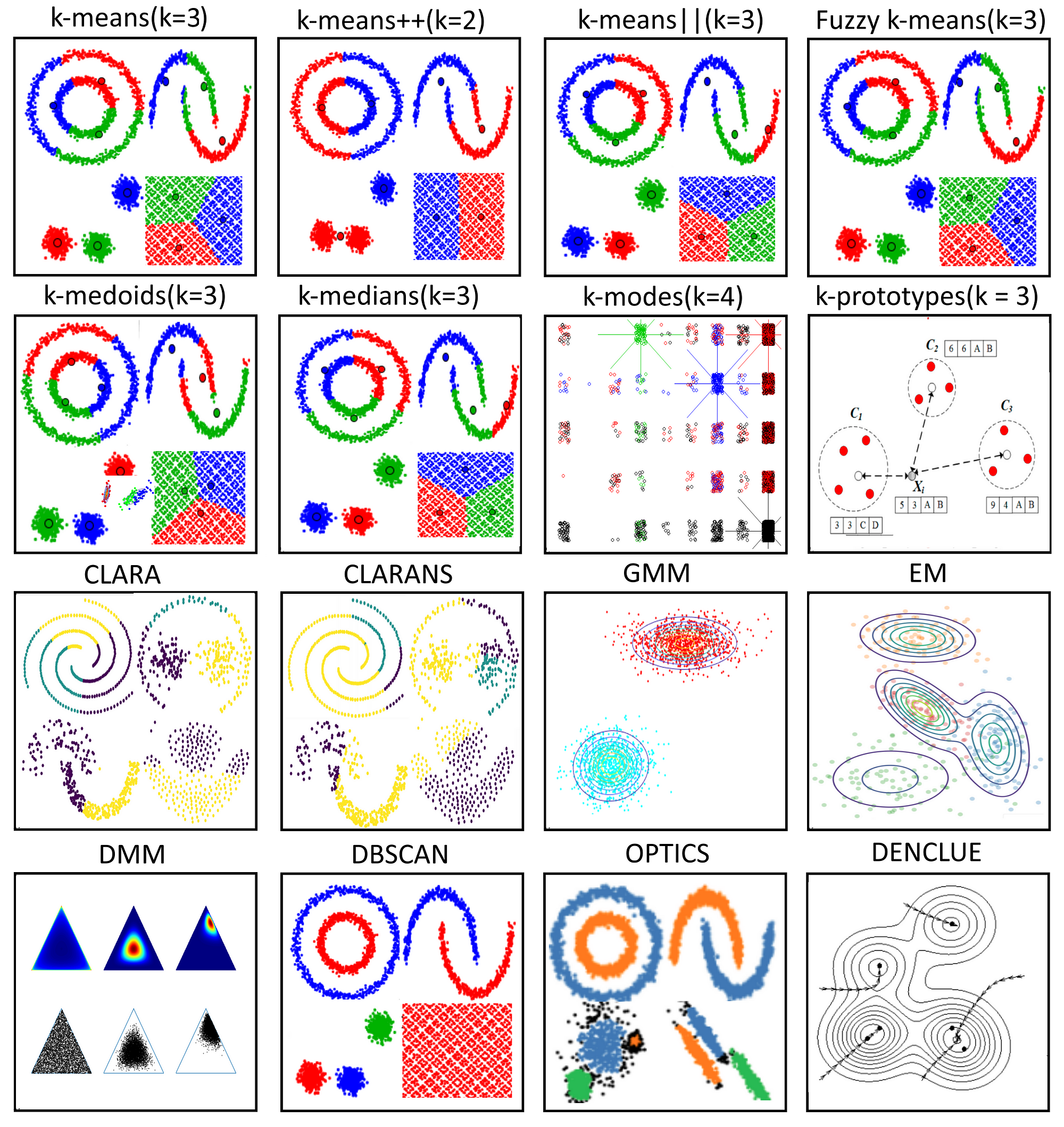
clustering algorithms

1. Partitioning Methods
- K-Means Clustering → divides the dataset into (k) clusters, where (k) is a predefined number of clusters (use when the no. of clusters is known or can be estimated)
- K-Medoids → uses medoids (actual data points) instead of centroids (more robust to noise and outliers)

2. Hierarchical Methods
- Agglomerative (bottom-up) → starts with each data point as a single cluster and iteratively merges the closest pairs of clusters
- Divisive (top-down) → starts with all data points in a single cluster and recursively splits them into smaller clusters

3. Density-based methods
- DBSCAN → groups data points into dense regions separated by regions of lower density
- OPTICS → extends DBSCAN by addressing its sensitivity to parameter selection

4. Model-based methods
- Gaussian Mixture Models (GMM)

5. Graph-Based Methods
- spectral clustering → uses the eigenvalues of the similarity matrix of the data to perform dimensionality reduction before clustering in fewer dimensions

6. Grid-Based Methods
- STING → divides the data space into a grid and performs clustering on the grid cells

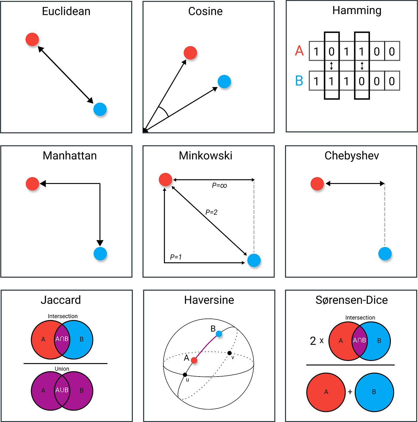
clustering distance measure

- defines how the similarity of two elements is calculated → influences the formation of clusters and how well the clustering algorithm performs

- Euclidean distance → straight-line distance btw two points in Euclidean space

- Manhattan distance → sum of the absolute differences of their coordinates

- Pearson correlation distance

Properties:
- Non-negativity
- Identity of indiscernibles
- Symmetry
- Triangle inequality

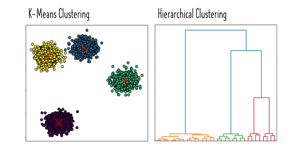
Hierarchical vs k-means clustering

- hierarchical clustering is an iterative method that builds a hierarchy of clusters either in a bottom-up manner or a top-down manner

- does not require specifying the number of clusters in advance

- produces a dendrogram → tree-like diagram showing the arrangement of clusters formed at each iteration

- more computationally intensive → suitable for smaller datasets where hierarchical relationships are important or the number of clusters is not known in advance

- K-means clustering partitions the dataset into (k) clusters, where (k) is a predefined number of clusters

- faster and more scalable than hierarchical clustering → suitable for larger datasets when the number of clusters is known or can be estimated

- sensitive to the initial placement of centroids

estimating clusters

- Elbow method → plotting the sum of squared distances (inertia) from each data point to its assigned cluster centroid as a function of k

- Information criterion approach → evaluating models with different numbers of clusters and selecting the model that optimizes a specific criterion

e.g. Akaike Information Criterion (AIC) → balances the goodness of fit of the model against its complexity

evaluating clustering

• Silhouette Coefficient

  • measures how similar an object is to its own cluster compared to other clusters

  • from -1 to +1 → higher value indicates better-defined clusters

• Dunn Index

  • The ratio of the minimum inter-cluster distance to the maximum intra-cluster distance

  • Higher values indicate better clustering

• Davies-Bouldin Index

  • average similarity ratio of each cluster with its most similar cluster

  • lower values indicate better clustering

• Calinski-Harabasz Index (Variance Ratio Criterion)

  • The ratio of between-cluster dispersion to within-cluster dispersion

  • higher values indicate better-defined clusters

• Adjusted Rand Index (ARI)

  • measures the similarity between two clusterings, often used when true labels are available

  • from -1 to 1, where 1 indicates perfect agreement

• Normalized Mutual Information (NMI)

  • measures the mutual information between the clustering result and true labels, normalized to a 0-1 range

  • higher values indicate better agreement with true labels

What is the purpose of evaluation?

1. Assessing Model Performance

• Accuracy: Determine how well the clustering algorithm has identified the underlying structure of the data.

• Quality: Measure the quality of the clusters formed, ensuring that they are meaningful and representative of the data.

2. Comparing Algorithms

• Benchmarking: Compare different clustering algorithms to identify which one performs best for a given dataset.

• Parameter Tuning: Evaluate the impact of different parameters on the performance of a clustering algorithm.

3. Understanding Data

• Insights: Gain insights into the data's structure, distribution, and inherent groupings.

• Validation: Validate assumptions about the data and the clustering results to ensure they are reliable and accurate.

4. Guiding Decisions

• Model Selection: Choose the most appropriate model or algorithm for a specific task based on evaluation results.

• Business Decisions: Inform business or scientific decisions based on the reliability and validity of the clustering results.

5. Improving Models

• Identify Weaknesses: Identify areas where the clustering algorithm may be underperforming and needs improvement.

• Optimize Performance: Fine-tune and optimize the algorithm to achieve better performance and more accurate clustering.

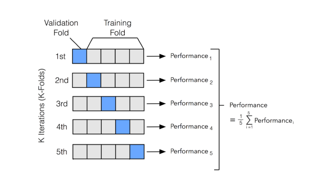
stratified k-fold cross-validation vs k-fold cross-validation

• k-fold cross-validation

  • the dataset is randomly divided into k equally (or nearly equally) sized subsets or "folds”

  • model is trained and validated k times, each time using a different fold as the validation set and the remaining k-1 folds as the training set

  • the final performance metrics is the avg of the performance metrics from each of the k iterations

• stratified k-fold cross-validation

  • similar but it maintains the original class distribution in each of the k subsets, making it more suitable for imbalanced classification problems

benchmarking

• benchmarking → systematically evaluating and comparing the performance of different algorithms or models using a standardized set of metrics and datasets

• understand the relative strengths and weaknesses of various approaches → provides a basis for selecting the most appropriate method for a given task

• establishes a baseline performance against which future models and improvements can be measured

neural network

• ML model inspired by the structure and function of the human brain

• structure → consists of layers of interconnected nodes/neurons that process and transmit information

• layers

  • input layer

  • hidden layer(s)

  • output layer

• learning → adjusting the strength of connections (weights) between nodes based on the error of their outputs compared to the desired outcome

• types

  • feedforward

  • convolutional

  • recurrent

• applications → various fields, from image and speech recognition to medical diagnosis

• advantages/benefits → handles complex, non-linear relationships, works with large amounts of data

• challenges → requires large amounts of data, computationally intensive, “black box” nature makes it difficult to interpret

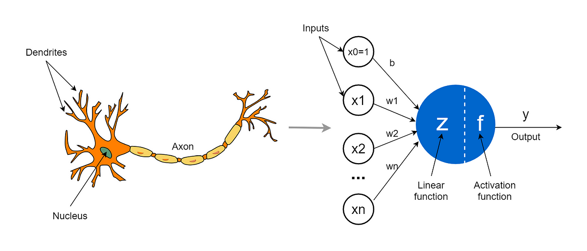
artificial neurons

• inputs (x₁, x₂, ..., xₙ)

• weights (w₁, w₂, ..., wₙ) → determine the importance of each input

• bias (b) → allows the neuron to shift its activation function

• summation function (Σ) → weighted sum of all inputs plus the bias

• activation function (f) → non-linear transformation of the summed input (determines whether/to what extent the neuron should "fire")

• output (y) → the result after applying the activation function (input to neurons in the next layer or as the final output)

neural network vs deep neural network

• depth of the network

  • neural networks have a few, while deep neural networks have many hidden layers

• capability

  • deep neural networks can model more complex functions and learn more abstract features, making them suitable for more complex tasks

• training and computation

  • deep neural networks typically require more data, longer training times, and more computational resources

In essence, deep neural networks are an extension of traditional neural networks, pushing the boundaries of what's possible in machine learning by leveraging increased depth and complexity.

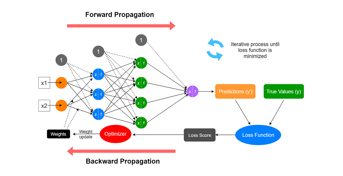
training of neural networks

• the learning process adjusts the network's parameters (weights and biases) to minimize the error between the predicted outputs and the actual target values

1. Training data → a collection of input-output pairs used to train the model

2. Initialization → the network's parameters (weights and biases) are set to small random values or based on specific initialization techniques

3. Forward Propagation → input data is passed through the network layer by layer, and each neuron processes the input by applying a weighted sum and a non-linear activation function

4. Loss Function → measures the difference btw the predicted outputs and the actual targets

5. Backpropagation → computing the gradient of the loss function with respect to each weight and bias in the network (these gradients indicate how much each parameter needs to change to reduce the loss)

6. Parameter update → weights and biases are updated by moving them in the direction that reduces the loss (step size is controlled by the learning rate parameter)

challenges in model training

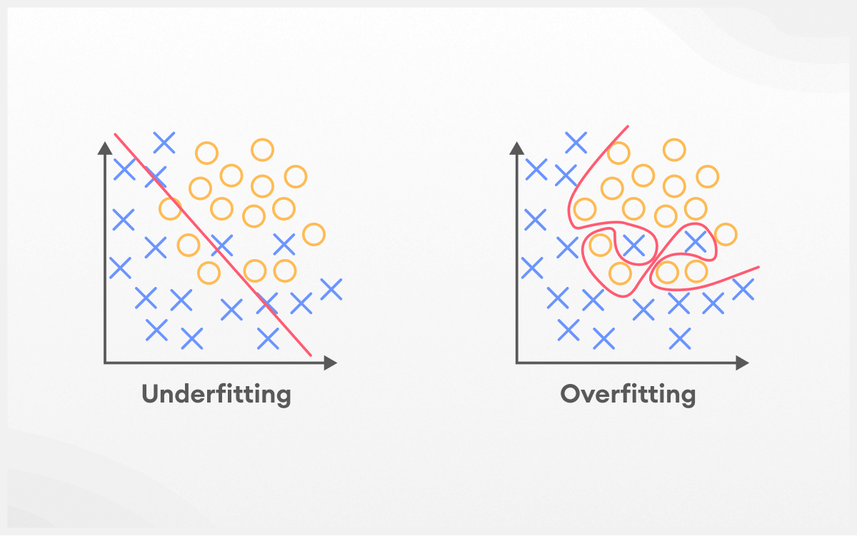
• Overfitting

  • the model learns the training data too well, including noise and outliers, which negatively impacts its performance on new data

• Underfitting

  • the model is too simple to capture the underlying patterns in the data, leading to poor performance on both training and new data.

• Hyperparameter Tuning

  • selecting optimal values for hyperparameters such as learning rate, number of hidden layers, number of neurons, batch size, etc.

• Computational Resources

  • training, especially for deep neural networks, can be computationally intensive and require significant hardware resources like GPUs

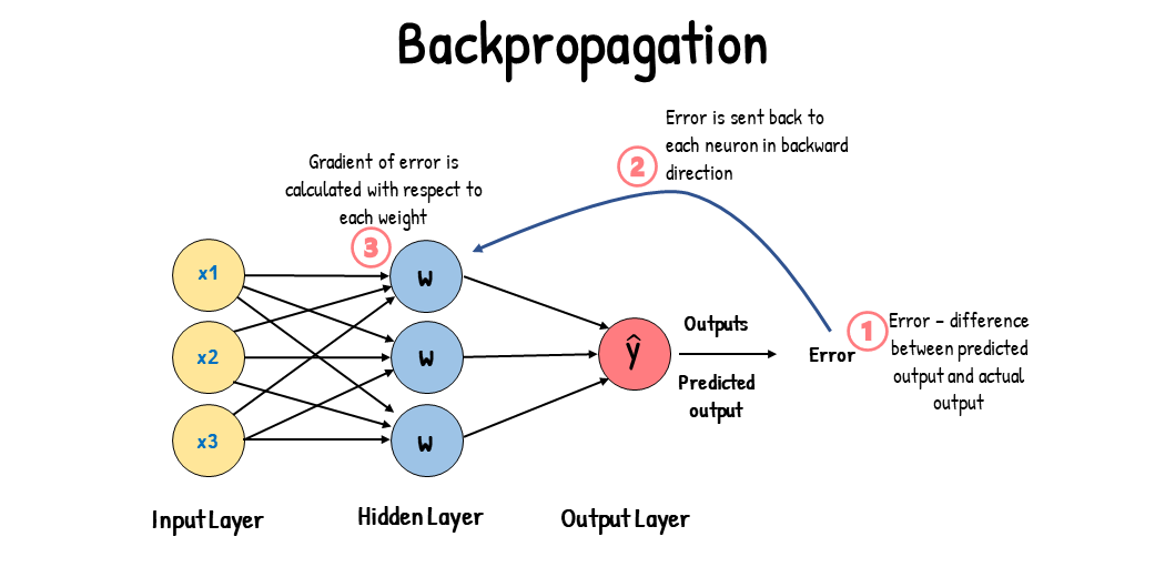
backpropagation

• the purpose of backpropagation is to optimize the neural network's parameters so that the error (loss) vtw the predicted and actual outputs is minimized

• initialization → computing the gradient of the loss function with respect to the output of the last layer →

• backward pass → computing the gradient of the loss with respect to each layer’s parameters by applying the chain rule of calculus

• parameter update → update the weights and biases using an optimization algorithm like gradient descent

How many hidden layers and neurons to use?

General Guidelines

• start simple → e.g. one hidden layer with a modes number of neurons

• evaluate the performance and gradually increase complexity (use grid search or random search to explore various configurations)

• domain knowledge → certain types of data often benefit from specific architectures

• problem complexity → more complex problems generally require deeper networks with more hidden layers

• no. of neurons → start with a number roughly btw the size of the input layer and the output layer (common practice is to use powers of 2 for easier computation)

• layer size decreasing → common heuristic is to have a decreasing no. of neurons in successive layers

Techniques

• cross-validation

• regularization

• hyperparameter tuning

• learning curves

• model selection

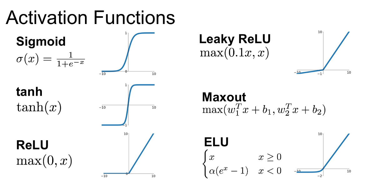
activation functions

• a function that calculates the output of the node based on its individual inputs and their weights

Activation functions for classification

• the goal is to assign an input to one of several classes

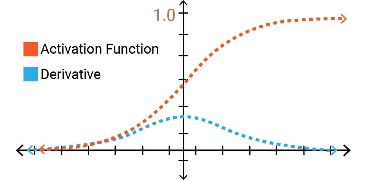
• Sigmoid function → used in the output layer for binary classification problems, where the output represents the probability of the positive class

• Softmax function → used in the output layer for multi-class classification problems, where each output neuron represents the probability of a specific class

• ReLU (Rectified Linear Unit) → used in hidden layers to introduce non-linearity and help the network learn complex patterns, but not used in the output layer for classification

Activation functions for regression

• the goal is to predict a continuous value

• Linear Activation Function

• ReLU (Rectified Linear Unit)

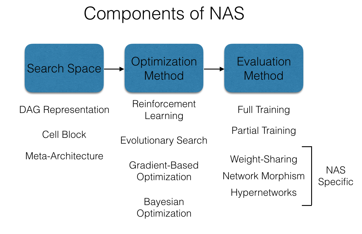
Neural Architecture Search (NAS)

• an automated process for designing the architecture of neural networks

  • find architectures that maximize performance metrics

  • optimize architectures for computational efficiency

  • automate the trial-and-error process of network design

• search space → define the set of all possible architectures that could be evaluated (no. of layers, types of layers, connectivity patterns etc.)

• search strategy → use algorithms to explore the search space

• performance evaluation → train and validate the proposed architectures to assess their performance

deep feed-forward neural network (DFNN)

• also known as a multilayer perceptron (MLP)

• a type of artificial neural network where connections between nodes do not form cycles, hence the term "feed-forward"

recurrent neural network (RNN)

• unlike feed-forward neural networks, RNNs have connections that form directed cycles, allowing information to persist over time

• RNNs are designed to work with sequential data

• RNNs are well-suited for tasks where context and order are important → time series prediction, language modeling, speech recognition

• the hidden state in an RNN serves as a memory that holds information from previous time steps

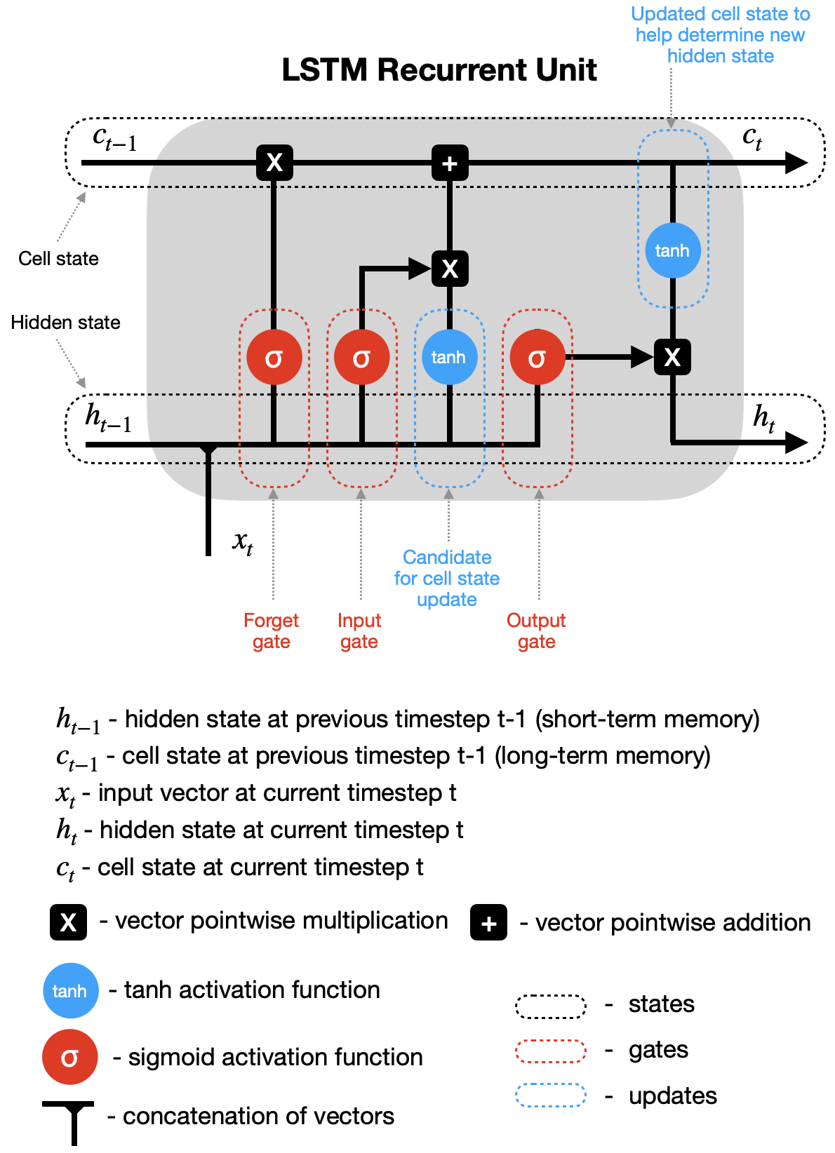
Long Short-Term Memory Network (LSTM)

• a special type of RNN designed to handle the vanishing and exploding gradient problems

• LSTMs have gates (input, forget, and output gates) that control the flow of information and maintain a cell state over time

  • forget gate → decides what information to discard from the cell state

  • input gate → decides which new information to add to the cell state

  • output gate → decides what part of the cell state to output as the hidden state

• cell state → acts as a conveyor belt, carrying information across many time steps with only minor linear interactions

• hidden state → the output of the LSTM unit at each time step

vanishing gradient problem

Occurs in deep neural networks when gradients become extremely small during backpropagation, leading to slow learning or convergence issues

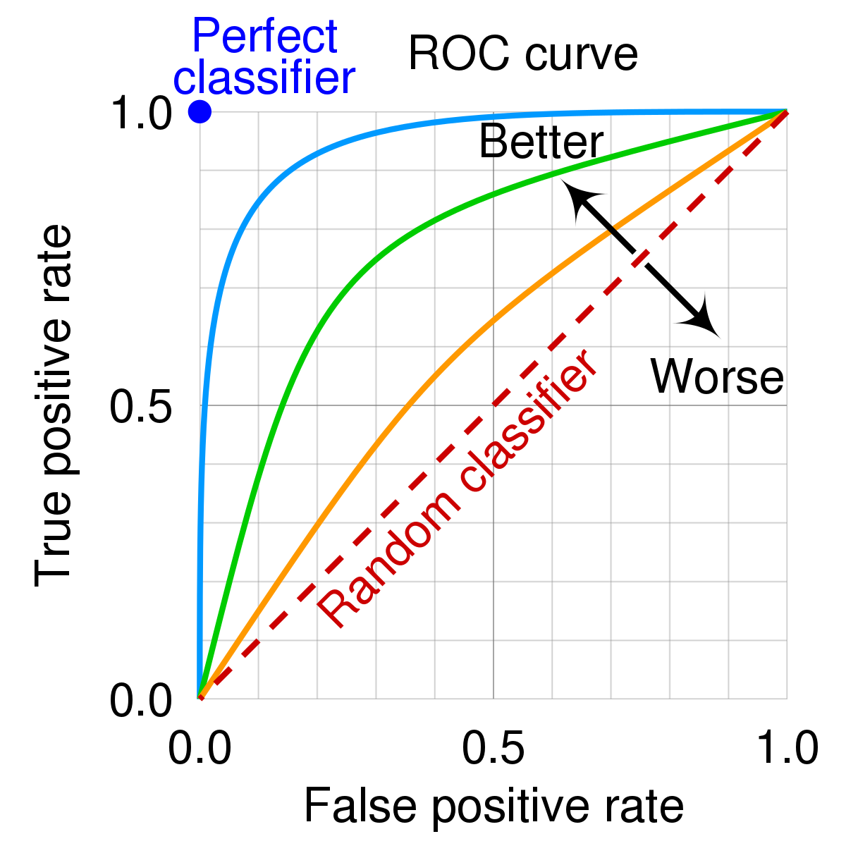
AUC - ROC curve

AUC → Area Under The Curve

ROC → Receiver Operating Characteristics

• used to measure performance of classification problems at various threshold settings

• ROC is a probability curve and AUC represents the degree or measure of separability

• The higher the AUC, the better the model is at classification

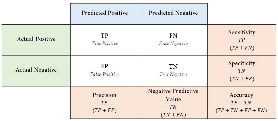
confusion matrix

• a table used to evaluate the performance of a classification model by displaying the number of true positives (TP), true negatives (TN), false positives (FP), and false negatives (FN)

transformers

• a type of a semi-supervised deep learning model → pre-trained in an unsupervised manner with a larger, unlabeled dataset, and then fine tuned through supervised training

Key components of a transformer model include:

• Attention Mechanism: self-attention mechanism allows the model to weigh the importance of different words in a sentence when encoding a particular word (enables the model to understand the context more effectively)

• Encoder-Decoder Architecture: The encoder processes the input data and encodes it into a set of continuous representations, while the decoder uses the encoded representations to generate the desired output

• Multi-Head Attention: several attention mechanisms running in parallel, which allows the model to focus on different aspects of the input simultaneously

• Positional Encoding: positional encodings are added to input embeddings to give the model information about the position of each word in the sequence

Popular transformer models:

• BERT

• GPT

• T5

• Transformer-XL

RNN vs LSTM vs transformers

• they are all types of neural network architectures that have been used to handle sequential data (e.g. time series, natural language text, and other ordered data)

Practical Use Cases:

- RNNs: Simple sequence tasks where the sequence length is not very long, such as basic time-series forecasting

- LSTMs: Applications requiring an understanding of long-term dependencies, like language modeling and speech recognition.

- Transformers: Tasks needing efficient handling of long sequences and complex dependencies, such as machine translation, text summarization, and other advanced NLP tasks

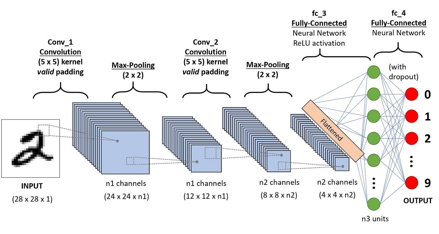
Convolutional Neural Network (CNN)

• type of deep learning model specifically designed to process structured grid data like images

• effective for tasks such as image classification, object detection, and other computer vision applications

Key components:

• Convolutional Layers

• Activation Functions

• Pooling Layers

• Fully Connected (Dense) Layers → where the actual classification or regression task is performed

• Dropout

• Feature Hierarchy

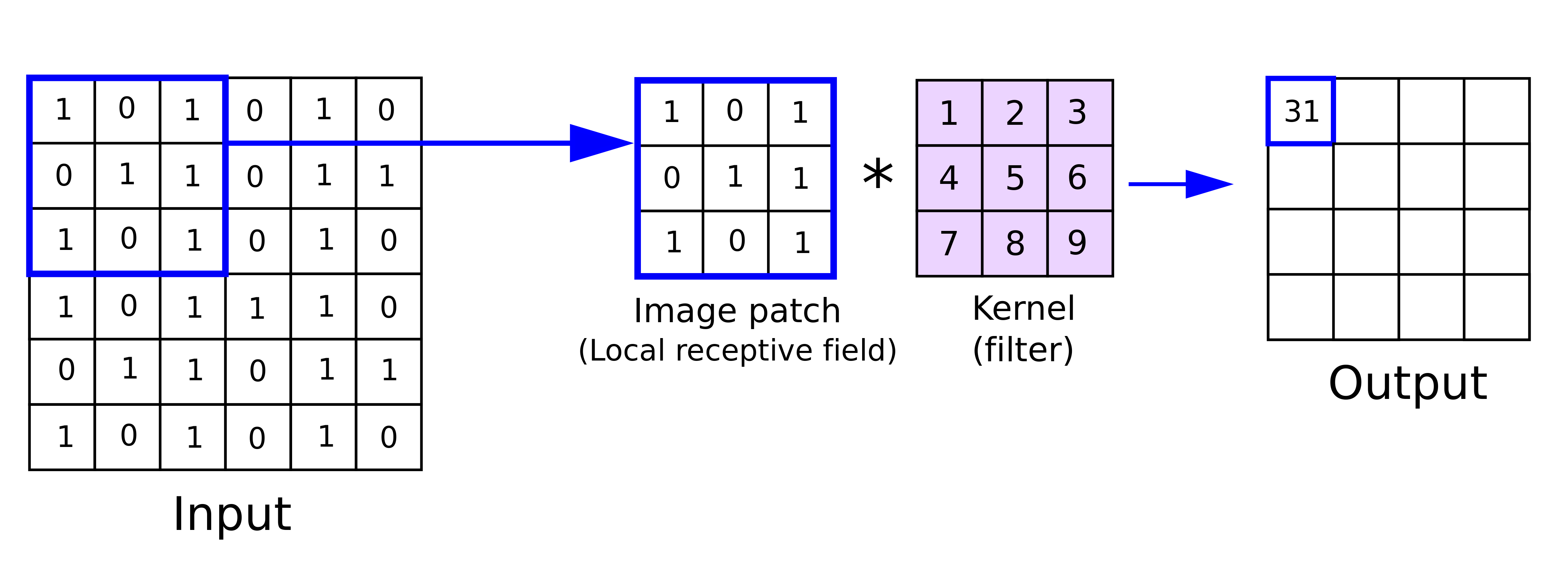
Convolutional Layers

• Convolution Operation: This layer applies a set of filters (also known as kernels) across the input image. Each filter slides over the input image (a process called "convolution") to produce an activation map, which highlights specific features such as edges, colors, or textures.

• Receptive Field: The area of the input image that a filter covers. By convolving, each filter looks at a small part of the image and creates a feature map.

Pooling Layers

• These layers perform a downsampling operation along the spatial dimensions (width, height), reducing the dimensionality of the feature maps while retaining the most significant information

• Common types of pooling include Max Pooling and Average Pooling

Dropout layer

A regularization technique where randomly selected neurons are ignored (dropped out) during training to help prevent overfitting.

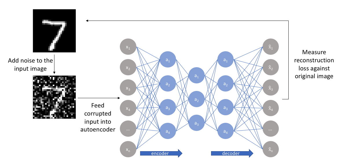
Autoencoders

• a type of artificial neural network used for unsupervised learning

• autoencoder network is designed to encode input data into a compressed and meaningful representation and then decode this representation back into data as similar as possible to the original input

• purpose → learn efficient representations of data for the purpose of dimensionality reduction or feature learning

Key components:

1. Encoder: compresses the input data into a smaller, encoded representation

2. Latent Space Representation (bottleneck): the central, most compressed layer that holds the encoded representation of the input

3. Decoder: reconstructs the original data from the encoded representation

Practical Use Cases:

• Dimensionality Reduction: Autoencoders can be used to reduce the dimensions of data, which is useful for visualization or as a preprocessing step for other machine learning algorithms.

• Feature Learning: They can automatically learn and extract important features from the data.

• Denoising: Autoencoders can learn to remove noise from data, e.g., image denoising.

• Anomaly Detection: By learning the normal pattern of data, autoencoders can help identify outliers or anomalies.

• Image Compression: They can compress images effectively while maintaining essential features.

• Generative Models: Variational Autoencoders (VAEs) are a type of autoencoder used for generating new data samples.

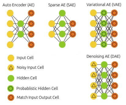
types of autoencoders

1. Basic autoencoders

2. Denoising autoencoders

3. Sparse autoencoders

4. Variational autoencoders (VAEs)

5. Convolutional autoencoders (CAEs)

6. Contractive autoencoders

7. Deep autoencoders

Key Differences:

• Purpose and Application: Each type of autoencoder is designed to handle specific tasks such as denoising, generating new data, or robust feature learning.

• Architecture: While the basic structure (encoder, latent space, decoder) remains similar, the specifics (e.g., layer type, noise addition, regularization) vary to meet the goals.

• Constraints and Regularizations: Types like sparse and contractive autoencoders introduce additional constraints to learn more meaningful or robust representations.

• Probabilistic Approach: VAEs introduce a probabilistic element to the latent space, enabling generative capabilities.

• Data Type: Convolutional autoencoders are specifically tailored for image data due to their convolutional layers.

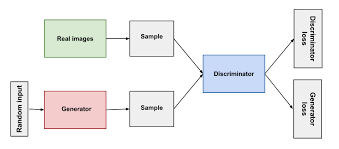
Generative Adversarial Network (GAN)

• a type of machine learning model used primarily for generating synthetic data that closely resembles real data

• consists of two neural networks:

  • generator → create synthetic data that mimics the real data

  • discriminator → distinguish between real data (from the training set) and fake data (produced by the generator)

  • trained simultaneously with competing objectives

• the ultimate goal of training a GAN is to reach a point where the generator produces data so realistic that the discriminator cannot reliably distinguish btw real and fake data

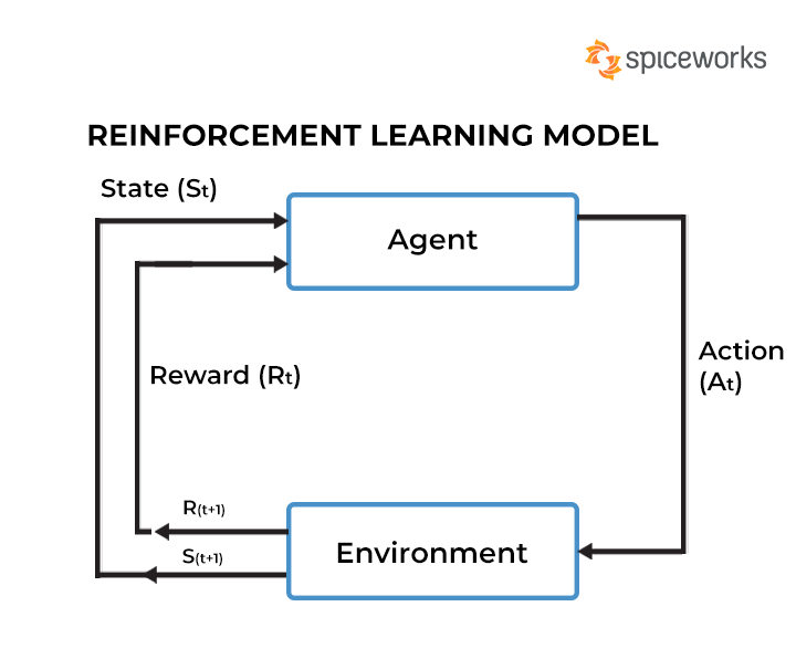
Reinforcement learning (RL)

• type of machine learning where an agent learns to make decisions by performing certain actions within an environment in order to maximize some notion of cumulative reward

• the goal of the agent is to learn a policy that maximizes the cumulative reward over time

Key components:

• Agent: The learner or decision maker.

• Environment: The external system with which the agent interacts.

• State (S): A representation of the current situation of the agent within the environment.

• Action (A): The set of all possible moves the agent can make.

• Reward (R): Feedback from the environment that evaluates the action taken by the agent.

RL entities

• various components that collectively define the learning environment and the overall learning process

Some of the primary entities in reinforcement learning include:

1. Agent: The learner or decision-maker that interacts with the environment. The agent takes actions based on a policy to maximize cumulative reward over time.

2. Environment: The external system with which the agent interacts. It provides feedback to the agent's actions in the form of rewards and new states.

3. State (s): A representation of the current situation or configuration of the environment. The state encompasses all the relevant information needed to make decisions.

4. Action (a): Choices or moves made by the agent. An action alters the state of the environment.

5. Policy (π): A strategy or rule that the agent follows to decide which action to take in a given state. It can be deterministic (a specific action is taken in each state) or stochastic (actions are taken according to a probability distribution).

6. Reward (r): A scalar feedback signal received by the agent after taking an action in a particular state. The reward indicates the immediate benefit (or cost) of the action.

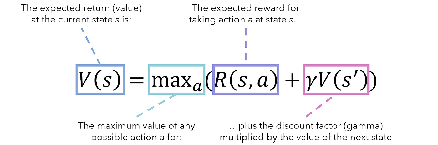
7. Value Function: A function that estimates the expected cumulative reward (or value) of being in a particular state. There are two main types:

   • State-value function (V(s)): Estimates the value of being in a state ( s ) and following a particular policy thereafter.

   • Action-value function (Q(s, a)): Estimates the value of taking an action ( a ) in a state ( s ) and following a particular policy thereafter.

8. Model: In model-based RL, the model encompasses the agent's understanding of the environment, typically in the form of transition probabilities (describing state transitions) and reward functions. It helps the agent to simulate and plan future actions.

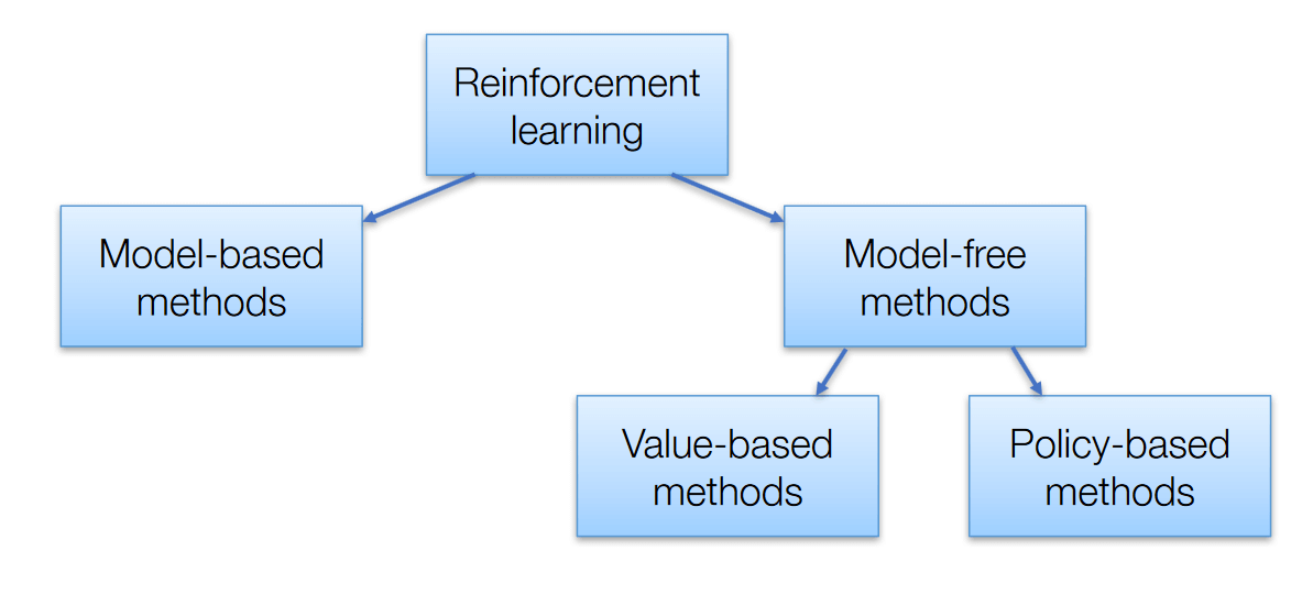
RL approaches

Model-Free vs. Model-Based

• Model-Free RL: The agent learns to make decisions without explicitly modeling the environment's dynamics. It relies entirely on experience gained through interaction with the environment.

  • Common algorithms include Q-learning and SARSA.

• Model-Based RL: The agent builds a model of the environment's dynamics (i.e., transition probabilities and reward functions). It uses this model to simulate and plan its actions.

  • Algorithms like Dyna-Q combine both model-free and model-based techniques.

Value-Based vs. Policy-Based vs. Actor-Critic Methods:

• Value-Based Methods: The agent learns a value function that estimates the expected cumulative reward for states or state-action pairs. Decisions are made by selecting actions that maximize the value.

  • Examples include Q-learning and Deep Q-Networks (DQN).

• Policy-Based Methods: The agent directly learns a policy that maps states to actions without explicitly learning a value function. These methods are useful in continuous action spaces.

  • Examples include REINFORCE and Proximal Policy Optimization (PPO).

• Actor-Critic Methods: These combine value-based and policy-based approaches. The actor learns the policy, while the critic evaluates the policy by learning the value function. This can stabilize and improve learning.

  • Examples include Asynchronous Advantage Actor-Critic (A3C) and Advantage Actor-Critic (A2C).

On-Policy vs. Off-Policy Learning:

• On-Policy Learning: The agent learns the value of the policy it is currently following. It evaluates and improves the same policy.

  • Examples include SARSA and some policy gradient methods like REINFORCE.

• Off-Policy Learning: The agent learns the value of a policy different from the one it is currently following. This allows the use of past experiences collected with different policies.

  • Examples include Q-learning and DQN.

Batch vs. Online Learning:

• Batch Learning: The agent learns from a batch of experiences collected during interactions with the environment, often stored in a replay buffer. This can improve sample efficiency and stability.

  • An example is the experience replay mechanism used in DQN.

• Online Learning: The agent updates its knowledge after each interaction with the environment. This can lead to faster adaptation but may be less stable.

Exploration vs. Exploitation Strategies:

• Exploration involves trying new actions to discover their effects and improve knowledge about the environment.

• Exploitation involves selecting the best-known actions to maximize the immediate reward.

• Common strategies to balance exploration and exploitation include ε-greedy (choosing random actions with probability ε), softmax (probabilistic action selection based on value estimates), and Upper Confidence Bound (UCB) methods.

Hierarchical Reinforcement Learning:

• This approach involves decomposing the learning task into a hierarchy of sub-tasks or skills. The agent learns policies at different levels of abstraction, which can simplify learning in complex environments. Examples include options framework and hierarchical DQNs.

Bellman equation

• the formula describes the relationship btw the value of a decision problem at a certain point in time and the value at subsequent points in time

• based on the principle of optimality → an optimal policy has the property that, whatever the initial state and initial decision are, the remaining decisions must constitute an optimal policy with regard to the state resulting from the initial decision

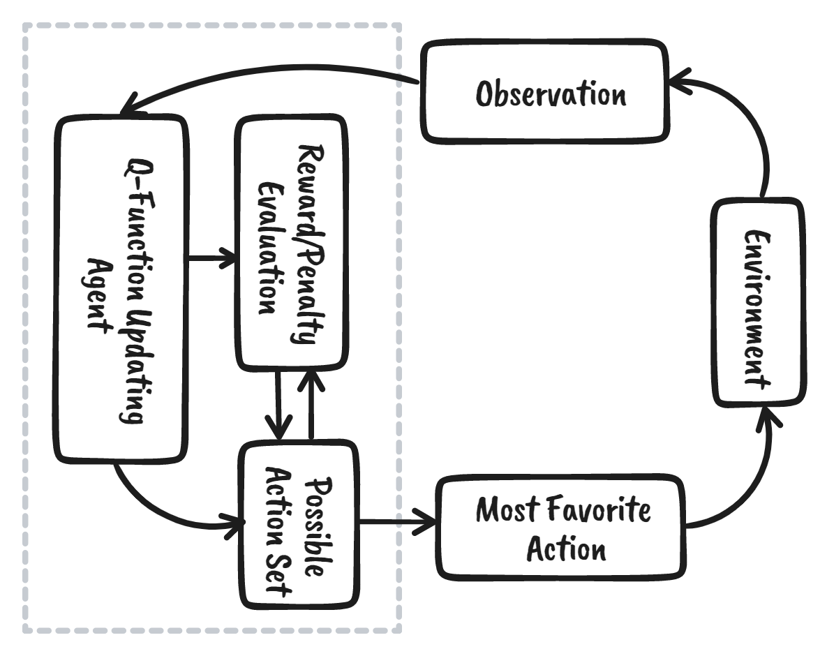
Q-Learning

• widely used algorithm in the field of reinforcement learning

• objective → learn the optimal policy that tells the agent the best action to take in each state to maximize its total cumulative reward

• updates the Q-values using the Bellman equation

• model-free → doesn't require a model of the environment and can be used in unknown environments

• off-policy → learns the optimal policy independent of the agent’s actions

Symbolic Learning

1. Representation: Uses symbols, rules, and logical structures to represent knowledge.

2. Reasoning: Employs explicit rules and logical inference for problem-solving.

3. Interpretability: Generally more interpretable and easier for humans to understand.

4. Knowledge acquisition: Often requires manual encoding of knowledge by experts.

5. Examples: Expert systems, decision trees, and rule-based systems.

6. Strengths: Good at handling abstract concepts and logical reasoning.

7. Weaknesses: Can struggle with uncertainty and handling large amounts of data.

symbolic vs sub-symbolic learning

1. Knowledge Representation:

   • Symbolic: Uses explicit symbols and rules.

   • Sub-symbolic: Uses distributed representations and numerical patterns.

2. Learning Process:

   • Symbolic: Often involves manual knowledge engineering.

   • Sub-symbolic: Typically involves automated learning from data.

3. Reasoning Mechanism:

   • Symbolic: Logical inference and rule application.

   • Sub-symbolic: Statistical inference and pattern matching.

4. Interpretability:

   • Symbolic: Generally more transparent and easier to interpret.

   • Sub-symbolic: Often less transparent, functioning as a "black box."

5. Handling Uncertainty:

   • Symbolic: Can struggle with uncertainty and probabilistic reasoning.

   • Sub-symbolic: Better at handling uncertainty and noisy data.

6. Scalability:

   • Symbolic: May face challenges with very large datasets.

   • Sub-symbolic: Generally scales well with large amounts of data.

7. Application Domains:

   • Symbolic: Often used in rule-based systems, expert systems, and formal reasoning.

   • Sub-symbolic: Commonly used in pattern recognition, computer vision, and natural language processing.

Sub-symbolic Learning

1. Representation: Uses numerical values, weights, and statistical patterns to represent knowledge.

2. Reasoning: Relies on statistical inference and pattern recognition for problem-solving.

3. Interpretability: Often less interpretable, functioning as a "black box."

4. Knowledge acquisition: Learns patterns from data automatically.

5. Examples: Neural networks, deep learning, and statistical machine learning algorithms.

6. Strengths: Excels at pattern recognition and handling large amounts of data.

7. Weaknesses: May struggle with abstract reasoning and explicit rule representation.

baseline model

• simple models that serve as a starting point for comparison with more complex models

• provide a benchmark performance → any model built should perform better than these baselines to be considered useful

Baseline Model in Classification:

• "Majority Class Classifier" (also known as "ZeroR" or "Most Frequent Class")

  • predicts the most frequent class in the training data for all instances in the test set

  • doesn't use any features/predictors for making predictions

Baseline Model in Regression:

• "Mean Model" (also known as "ZeroR" for regression)

  • calculates the mean of the target variable in the training data

  • predicts this mean value for all instances in the test set

  • doesn't use any features/predictors

subgroup discovery

• data mining and ML technique that aims to find interesting and interpretable patterns or rules that describe subsets of a dataset

• objective → identify subgroups that are both statistically significant and potentially actionable/interesting from a domain perspective

• some popular algorithms include:

  • PRIM, CN2-SD, SD-Map, DSSD

relational learning

• subfield of machine learning that focuses on learning and reasoning about data with complex relational structures → datasets where entities are interconnected and have multiple types of relationships

semantic data mining

• advanced approach to data mining that incorporates semantic information, ontologies, and domain knowledge into the data analysis process

• semantic annotation → data is enriched with semantic tags or metadata to provide context and meaning

• promotes multi-modal data integration

heuristics

• problem-solving techniques or rules of thumb that are used to find approximate solutions quickly when exact methods are too slow or impractical

• often used in optimization problems to find good (but not necessarily optimal) solutions efficiently

• in AI systems, heuristics can be employed to mimic human-like decision-making processes

entropy

• measure of the average amount of information contained in a message

• in the context of ML, it quantifies the impurity or uncertainty in a set of examples

information gain

• the reduction in entropy (or increase in information) that results from splitting a dataset according to a particular feature

• crucial concept in decision tree algorithms for selecting the best feature to split on at each node

overfitting

• when a model learns the training data too well, including its noise and peculiarities, to the point that it performs poorly on new, unseen data

How to identify overfitting?

• a significant difference btw the model's performance on training data and validation/test data indicates overfitting

• model is unnecessarily complex for the given problem

• training error continues to decrease while validation error starts to increase

• model gives high importance to irrelevant features

Methods to deal with overfitting:

• cross-validation → use techniques like k-fold cross-validation to get a more robust estimate of model performance

• increasing the amount of training data can help the model learn more general patterns

• remove irrelevant/redundant features that might be contributing to overfitting

• regularization → penalty term for the loss function to discourage complex models

• early stopping → stop training when the model's performance on a validation set starts to degrade

• ensemble methods → combining predictions from multiple models to reduce overfitting

• domain expertise → incorporate domain knowledge to guide feature engineering and model selection

underfitting

• when a model is too simple to capture the underlying patterns in the data

How to identify underfitting?

• the model performs poorly on both training and validation/test data

• high bias → model consistently misses important patterns in the data

• oversimplification → model makes overly simplistic assumptions about the data

• similar error rates → training and validation errors are similar but both are high

• both training and validation errors remain high and do not improve significantly with more data

• residual analysis → for regression problems, residuals show clear patterns, indicating that the model hasn't captured important relationships

Methods to deal with underfitting:

• using a more sophisticated model that can capture more complex patterns in the data

• adding additional relevant features that might help explain the target variable

• feature engineering → creating new features or transforming existing ones to better represent the underlying patterns

• reduce regularization

• ensemble methods → combine multiple simple models to create a more powerful predictive model

• polynomial features → for linear models, add polynomial terms to capture non-linear relationships

• domain expertise → incorporate domain knowledge to guide feature engineering and model selection

• hyperparameter tuning → optimize the hyperparameters of your model to find the best configuration

association rule learning

• a data mining and ML technique used to discover interesting relationships or patterns among variables in large datasets