stats

Scales of measurement

Ways to categorize different types of data: binary, nominal, ordinal, interval, and ratio scales.

binary

• Definition: A scale with only two possible values, typically representing the presence/absence or true/false of a characteristic.

• Key Feature: Only two categories.

• Examples:

  • Gender (in binary terms): Male = 0, Female = 1

  • Response to a yes/no question: Yes = 1, No = 0

  • Pass/Fail outcome

nominal

• Definition: A categorical scale where values are names or labels without any quantitative value or order.

• Key Feature: Categories have no inherent order.

• Examples:

  • Types of fruits: Apple, Orange, Banana

  • Blood types: A, B, AB, O

  • Marital status: Single, Married, Divorced

ordinal

• Definition: A scale where values can be ranked or ordered, but the intervals between them are not necessarily equal.

• Key Feature: Order matters, but distances are not consistent.

• Examples:

  • Customer satisfaction: Very Unsatisfied, Unsatisfied, Neutral, Satisfied, Very Satisfied

  • Education level: High School < Bachelor’s < Master’s < Doctorate

  • Movie ratings: 1 star, 2 stars, 3 stars...

interval

• Definition: A numeric scale where both order and exact differences between values are meaningful, but there is no true zero point.

• Key Feature: Equal intervals, no absolute zero.

• Examples:

  • Temperature in Celsius or Fahrenheit (0°C does not mean “no temperature”)

  • Dates in the calendar (e.g., 2000, 2010—differences matter, but year 0 is arbitrary)

ratio

• Definition: A numeric scale with all the properties of an interval scale, and it includes a true zero point, allowing for meaningful ratios.

• Key Feature: True zero, so ratios make sense (e.g., 10 is twice as much as 5).

• Examples:

  • Height, Weight, Age, Length, Income

  • Number of children in a family (0 means no children)

Types of reliability

Consistency of a measure; includes test-retest, inter-rater, and internal consistency reliability.

Test-Retest Reliability

• Definition: The consistency of a measure over time—whether a test gives similar results when taken by the same individuals at two different points in time.

• Key Feature: Stability across time.

• Example:

  • A personality test is administered to the same group of people two weeks apart. If the results are similar, the test has high test-retest reliability.

Inter-Rater Reliability

• Definition: The degree of agreement among different observers or raters measuring the same thing.

• Key Feature: Consistency between observers.

• Example:

  • Two judges rating the performance of gymnasts in a competition. If their scores are similar, inter-rater reliability is high.

Intra-Rater Reliability

• Definition: The consistency of results across items within a test—whether items intended to measure the same construct yield similar results.

• Key Feature: Consistency within the test itself.

• Common Statistic: Cronbach’s alpha

• Example:

  • A depression scale with 10 items. If all items correlate well with each other, the scale has high internal consistency.

Parallel Forms Reliability (Alternate Forms)

• Definition: The consistency of results between two different versions of the same test administered to the same group.

• Key Feature: Different forms, same concept.

• Example:

  • Students take two versions of a math test that are supposed to be equivalent. If scores are similar, parallel forms reliability is high.

Split-Half Reliability

• Definition: A measure of internal consistency where the test is split into two halves, and the scores on both halves are compared.

• Key Feature: Measures internal consistency with fewer computations than Cronbach’s alpha.

• Example:

  • A 20-question test is split into two sets of 10. If scores on both halves are similar, the test has good split-half reliability.

Types of validity

Accuracy of a measure; includes content, construct, and criterion-related validity.

face validity

• Definition: The extent to which a test appears to measure what it’s supposed to, at face value.

• Key Feature: Based on subjective judgment, not statistical analysis.

• Example:

  • A math test that includes only math problems has high face validity. But if it includes unrelated word puzzles, it would lack face validity.

Content Validity

• Definition: The extent to which a test covers the entire range of the concept or domain it's intended to measure.

• Key Feature: Assessed by expert judgment.

• Example:

  • An English grammar test that includes all key grammar topics (tenses, punctuation, syntax) has high content validity.

Construct Validity

• Definition: The extent to which a test truly measures the theoretical construct it's intended to measure.

• Key Feature: Involves both convergent and discriminant validity.

• Example:

  • A new scale designed to measure anxiety should correlate with other anxiety measures (convergent validity) and not correlate with unrelated constructs like physical strength (discriminant validity).

Criterion Validity

• Definition: The extent to which a test correlates with a relevant outcome or criterion.

• Subtypes:

  • Concurrent Validity: Correlation with a current outcome.

  • Predictive Validity: Correlation with a future outcome.

• Example:

  • Concurrent: A job skills test that correlates with current employee performance.

  • Predictive: SAT scores predicting college GPA.

Ecological Validity

• Definition: The extent to which research findings or test results generalize to real-world settings.

• Key Feature: Real-life applicability.

• Example:

  • A memory test conducted in a classroom that reflects how students actually learn and recall information.

External Validity

• Definition: The extent to which the results of a study can be generalized to other populations, settings, or times.

• Example:

  • A psychological experiment on college students that can also be generalized to adults in the workforce.

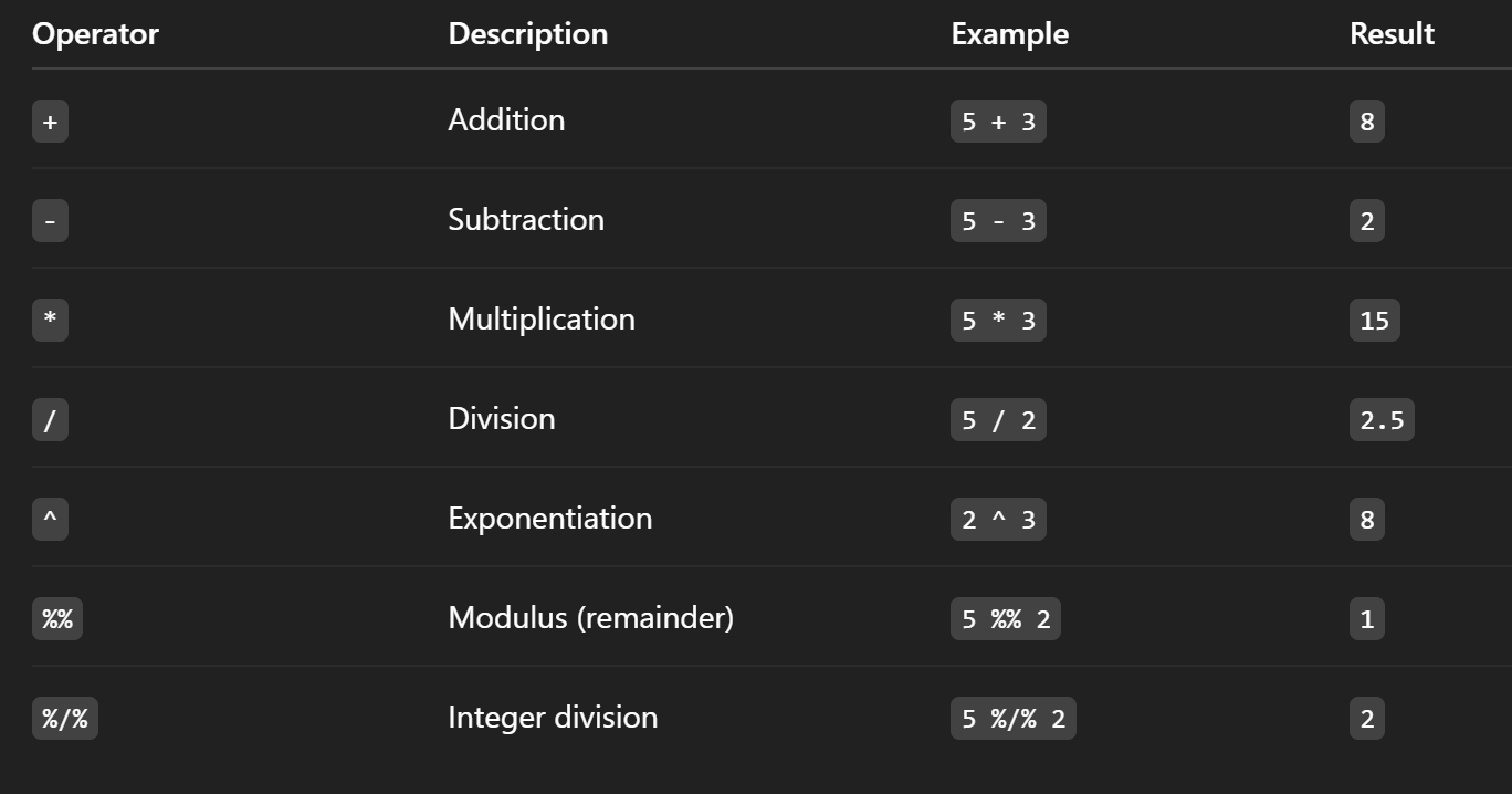
Arithmetic operators

Symbols used in R for basic math: +, -, *, /, ^, %%, %/%.

Logical operators

Symbols for logical comparisons in R:

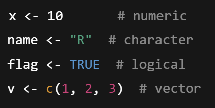
Variables

Named storage for data in R; can be numeric, character, logical, or vectors.

Functions and arguments

Reusable code blocks with inputs (arguments) to perform tasks in R.

Special values in R

Inf (infinity)

NA (Not Available ): Represents a missing or undefined value in a vector or dataset

NaN (Not a Number): A numeric value that results from undefined mathematical operations, such as 0/0 or Inf - Inf.

NULL: Represents the absence of a value or object entirely.

Vectors and indexing

One-dimensional arrays in R, accessed via [index].

Reading in data files

Importing data into R using functions like read.csv().

Data frames and matrices

Two-dimensional data structures in R; subset using [rows, columns].

Installing/loading packages

Use install.packages() and library() to add and use external R libraries.

Saving/loading workspaces

Use save.image() and load() to preserve and restore R environments.

Summarizing data frames

Use functions like summary(), str(), head() to inspect R data frames.

Mean

Average value of a data set; sum of values divided by number of values.

Median

Middle value when data are ordered; resistant to outliers.

Mode

Most frequently occurring value(s) in a dataset.

Variance

Average of the squared deviations from the mean.

Standard deviation

Square root of variance; measures spread around the mean.

Range

Difference between the highest and lowest values.

IQR

IQR = Q3 - Q1

Interquartile range; difference between the 75th (q3) and 25th (q1) percentiles.

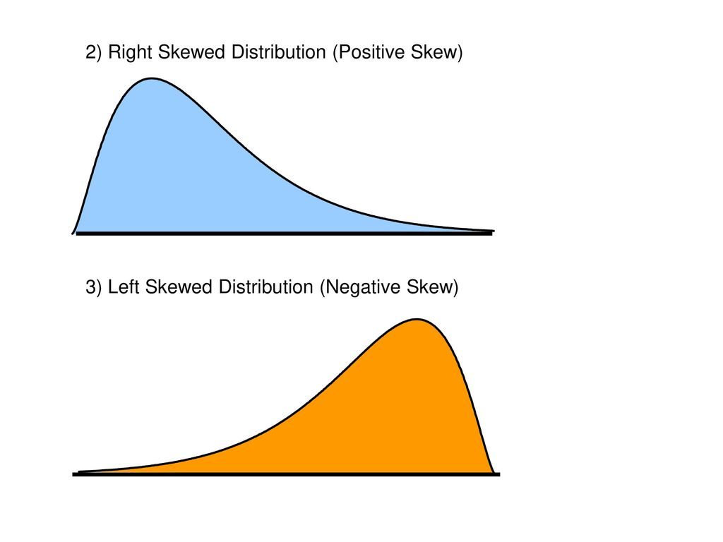
Skewness

Measure of asymmetry of the distribution.

positively skewed (right skewed)

negativly skewed (left skewed )

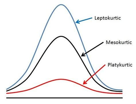
Kurtosis

Measure of peakedness or tail weight of the distribution.

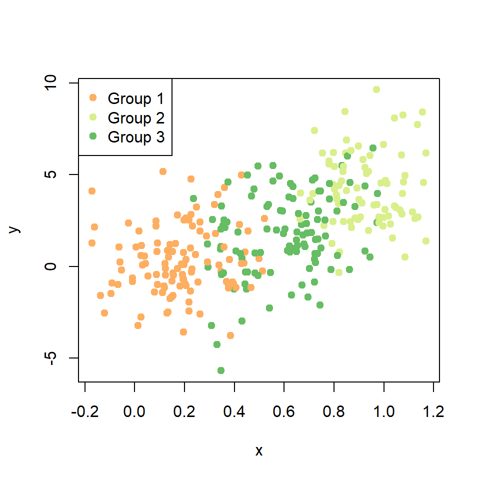
Correlation

Statistical measure of the relationship between two variables.

Scatter plot

Graph showing relationship between two continuous variables.

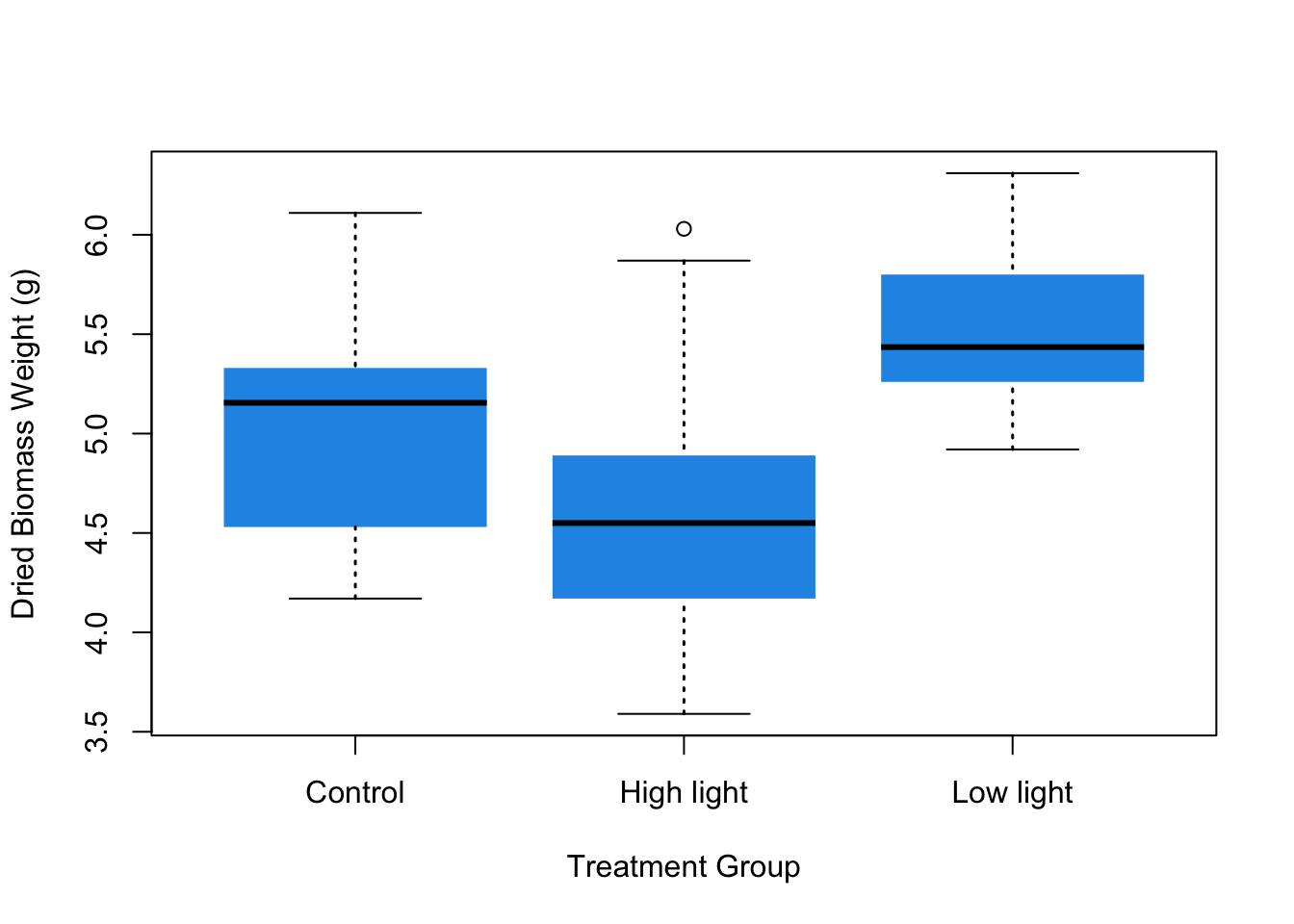
Box plot

Shows median, quartiles, and potential outliers of a dataset.

box plots only show the median not the mean

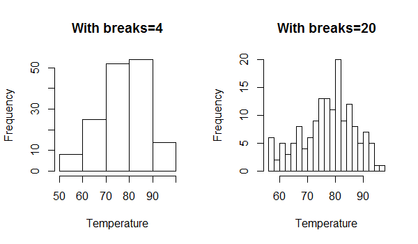
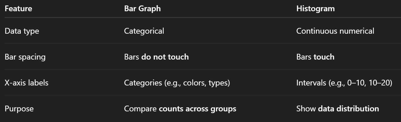
Histogram

Bar graph showing frequency of numeric data ranges.

Bar graph

Displays categorical data with rectangular bars.

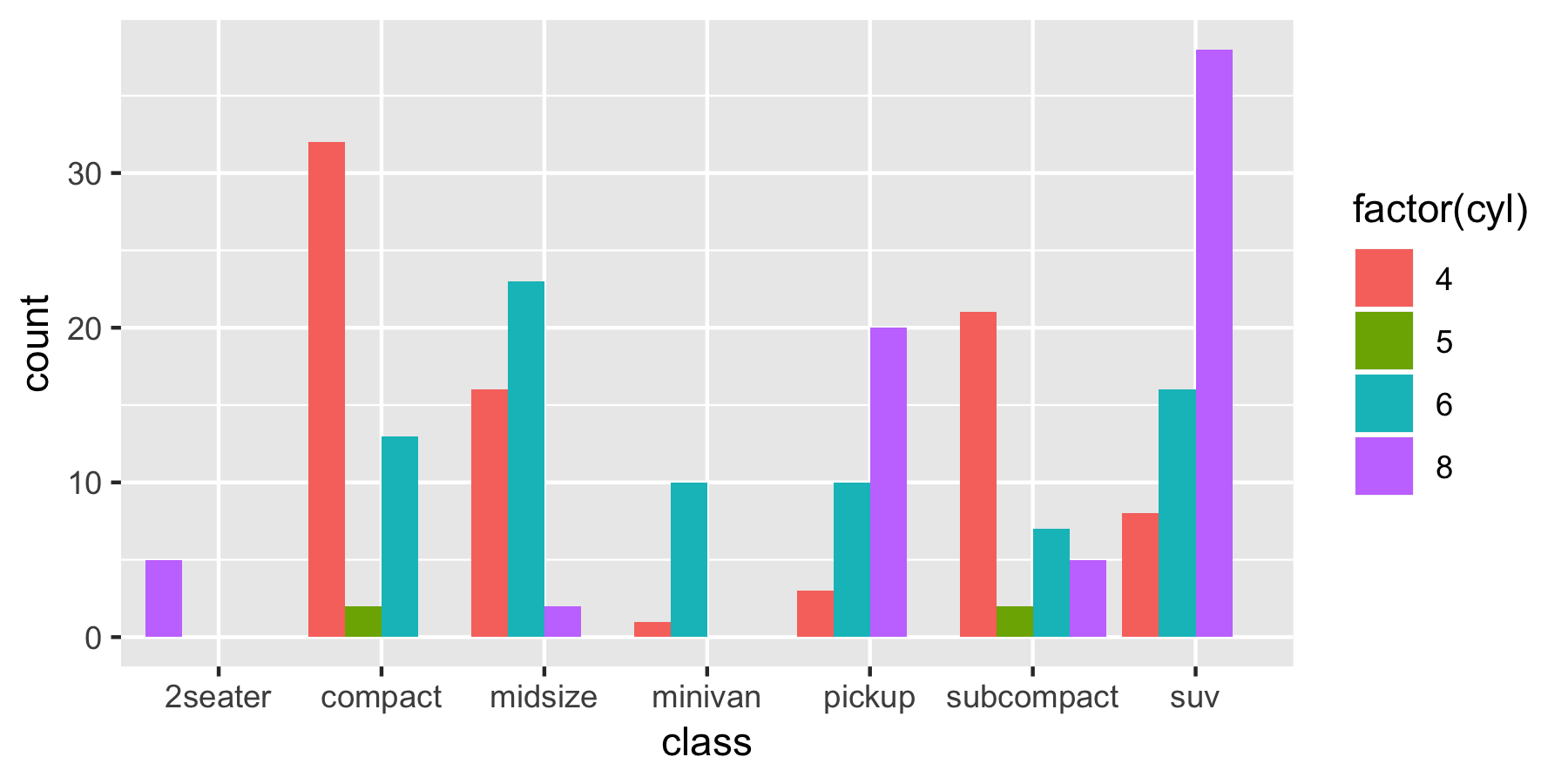
difference bar graph and histogram

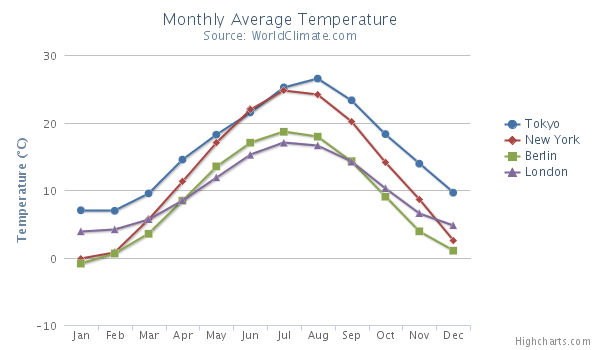
Line graph

Shows trends over time or ordered categories.

Null hypothesis

Statement that there is no effect or difference.

Alternative hypothesis

Statement that there is an effect or difference.

P-value

The p-value is the probability of obtaining results as extreme as, or more extreme than, the observed results, assuming the null hypothesis is true.

Alpha level

Threshold probability for rejecting the null hypothesis, often 0.05.

a>=p → reject null, a < p → support null

steps in a test of significance.

1. state the hypothesis

2. set the level of risk (alpha level)

3. select the appropriate test statistic

4. compute the test statistic

5. state if the result rejected/failed to reject the null hypothesis

    

Two-tailed p-value = 2 × one-tailed p-value, if the test statistic is symmetric and the test is two-sided.

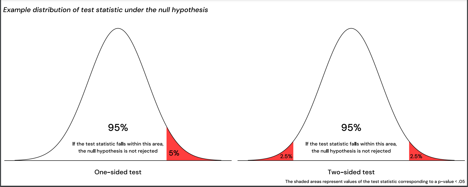
Rejection region

The rejection region is the range of values in a statistical test where, if your test statistic falls within it, you reject the null hypothesis.

Confidence interval

A confidence interval (CI) is a range of values that is likely to contain the true population parameter (like the mean), based on your sample data.

Sampling distribution

Distribution of a statistic over many samples.

Standard error

Standard deviation of the sampling distribution.

Central Limit Theorem

States that the sampling distribution of the mean approaches normality as sample size increases.

Type I error

False positive; rejecting the null hypothesis when it is true.

Type II error

False negative; failing to reject the null hypothesis when it is false.

Statistical power

Probability of correctly rejecting a false null hypothesis.

Degrees of freedom

Number of values free to vary in calculation after constraints are applied.

Imagine a Simple Puzzle

Let’s say you're arranging 3 numbers so that their average must be 10.

• You pick the first number: say, 8. You're free.

• You pick the second: maybe 12. Still free.

• But now the third? You’re not free anymore — it must be 10 to make the average exactly 10.

So:
🟢 1st number: free to choose
🟢 2nd number: free to choose
🔴 3rd number: locked in — depends on the others

👉 You had 2 degrees of freedom — two values could vary freely, the third was constrained.

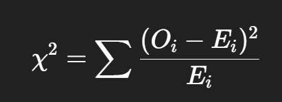
(chi-sqaur) χ² Goodness-of-Fit Test

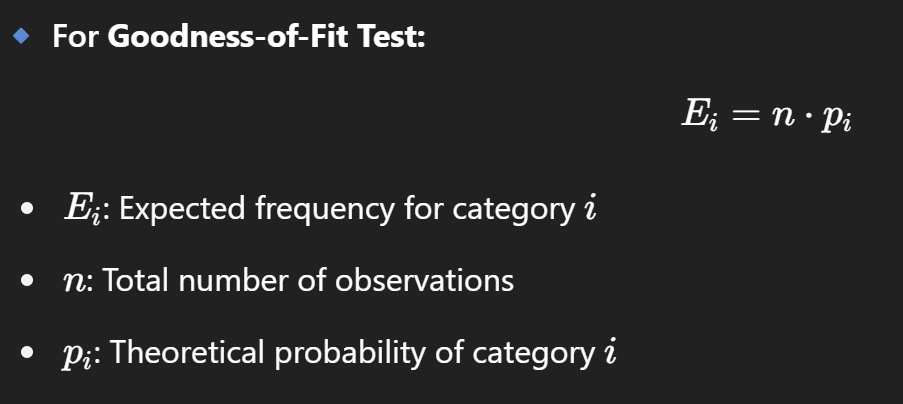
To test if an observed frequency distribution fits an expected (theoretical) distribution.

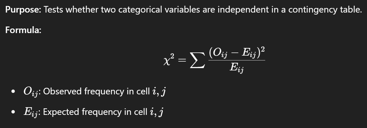
Oi = Observed frequency in cell i

Ei = Expected frequency in cell i

expected frequency for (chi-sqaur) χ² Goodness-of-Fit Test

(chi-square) χ² Test of Independence

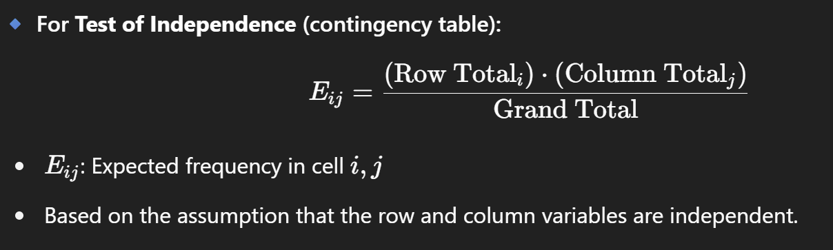
expected frequency for (chi-sqaur) χ² Test of Independence

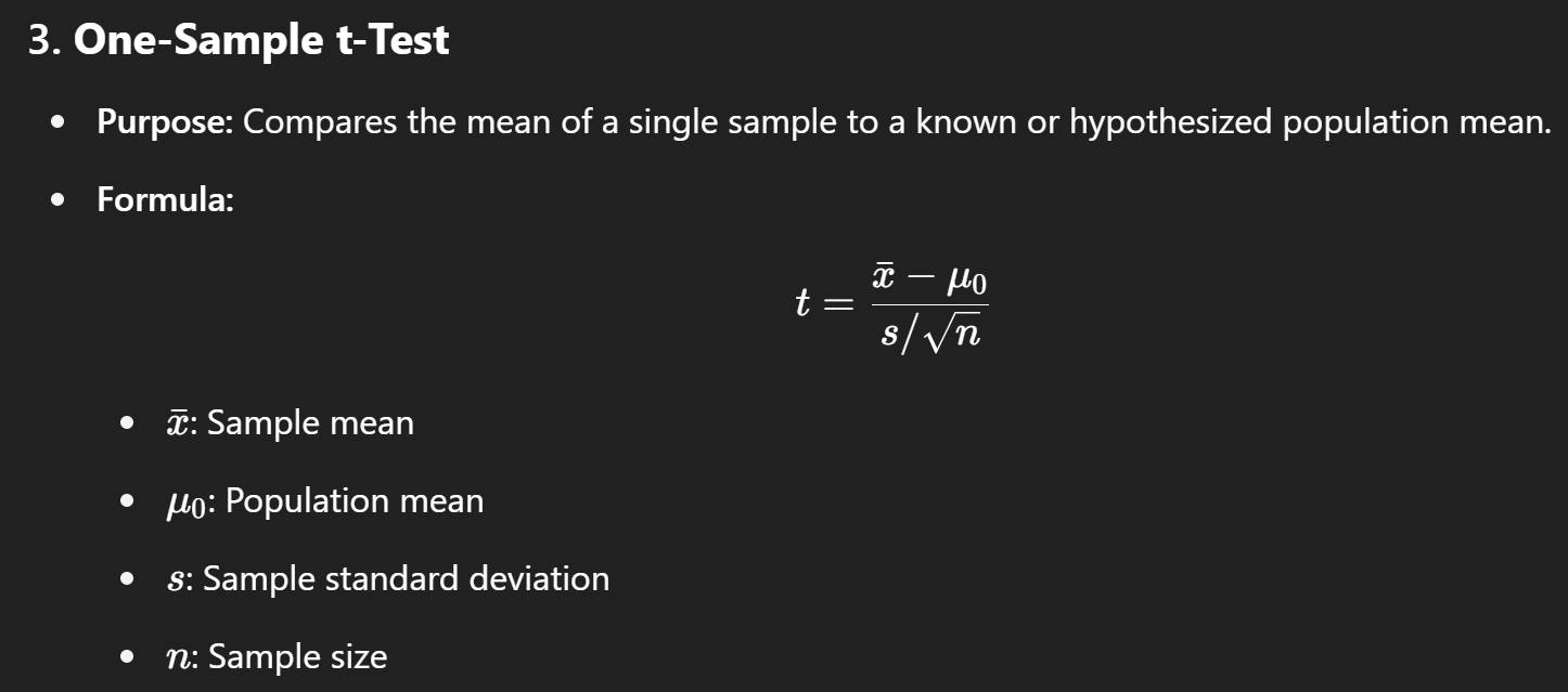
one sample t test

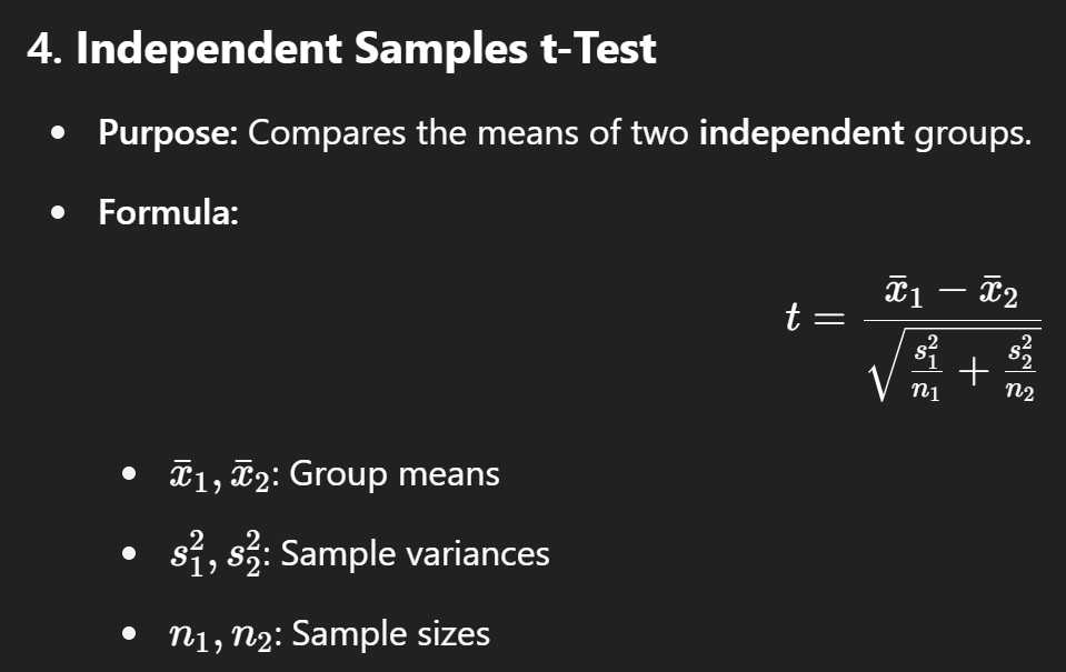
independent samples t test

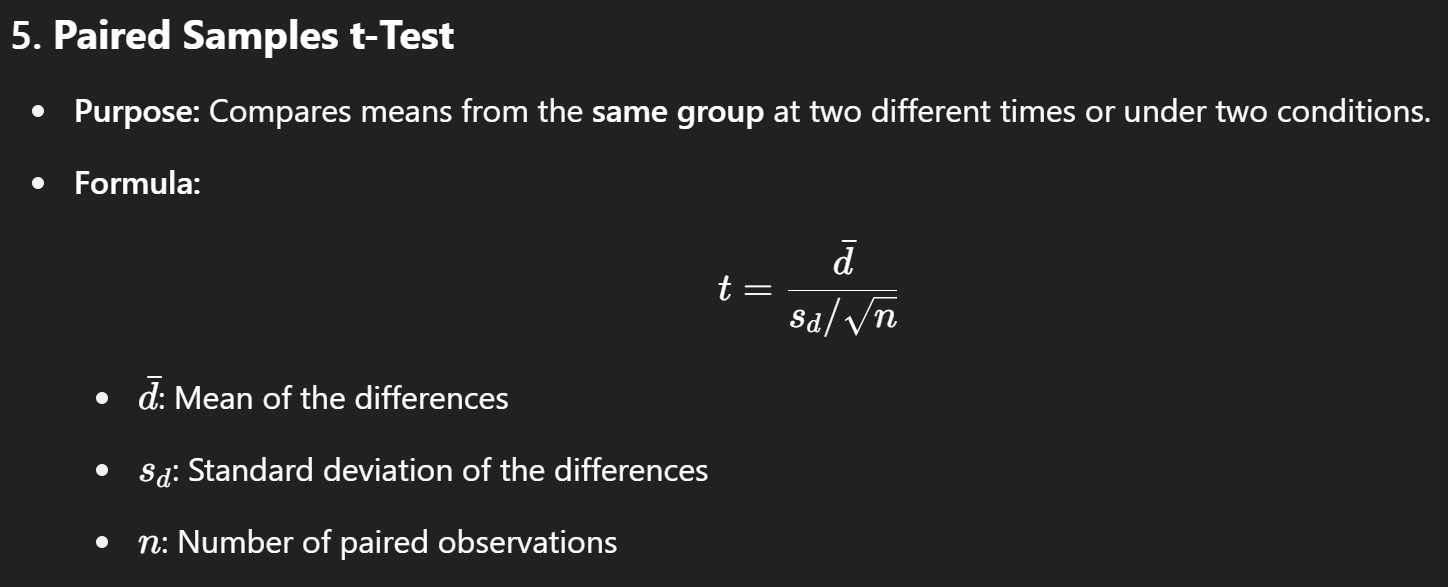
paired sample t test

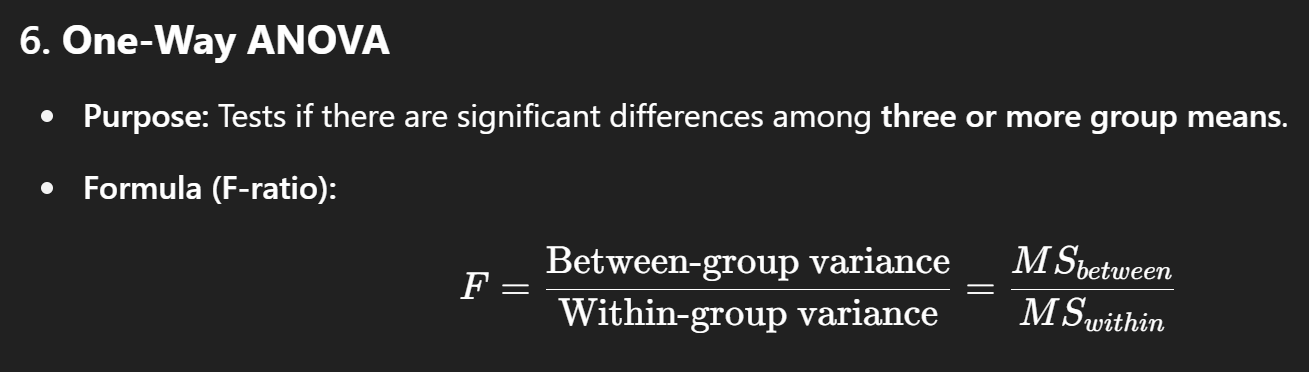
one way anova

• sort t-test for more variables

• Between-group variance: How much group means vary from the overall mean

• Within-group variance: How much values within each group vary from their own group mean

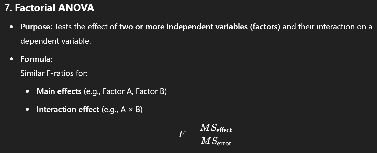
factorial anova

Degrees of freedom of χ² Goodness-of-Fit Test

df=k−1

Where k is the number of categories. You subtract 1 because once all but one category are known, the last is determined (due to the total sum constraint).

Degrees of freedom of χ² Test of Independence

df=(r−1)(c−1)

Where r = number of rows and c = number of columns in the contingency table. This measures how much freedom there is to vary cell values independently while keeping row and column totals fixed.

Degrees of freedom of One-Sample t-Test

df=n−1

Where nnn is the sample size. We lose one degree of freedom because we estimate the mean from the sample.

Degrees of freedom of Independent Samples t-Test (equal variances)

df=n1​+n2​−2

Where n1​ and n2​ are the sizes of the two groups. We subtract 2 because we estimate one mean and one variance per group.

Degrees of freedom of Paired Samples t-Test

df=n−1

Where nnn is the number of pairs. Only the differences are used, so it's treated like a one-sample t-test on the difference scores.

Degrees of freedom of One-Way ANOVA

• Between groups:

  dfbetween = k−1

• Within groups (error):

  dfwithin= N−k

Where k = number of groups, and N = total number of observations

Degrees of freedom of Factorial ANOVA (2 factors A and B)

• Main effect A:

  dfA = a−1

• Main effect B:

  dfB = b−1

• Interaction A × B:

  dfA×B = (a−1)(b−1)

• Error (within):

  dferror = N−ab

Where a and b are the number of levels in each factor and N is total observations.

Shapiro-Wilk Test

Shapiro-Wilk Test checks whether a sample comes from a normally distributed population.
Purpose: Tests for normality of data.

• Null Hypothesis (H₀): The data is normally distributed.

• Alternative Hypothesis (H₁): The data is not normally distributed.

• Test Statistic: W (ranges between 0 and 1).

• Interpretation:

  • If p > 0.05 → Fail to reject H₀ → Data likely normal.

  • If p ≤ 0.05 → Reject H₀ → Data likely not normal.

• Sample Size: Best for small to moderate samples (n < 2000).

F-test

F-test is used to compare variances between two populations or to test the overall significance of a regression model.

• Common Uses:

  1. Variance Comparison:

     • Tests if two samples have equal variances.

     • Often a pre-test for t-tests that assume equal variance.

  2. ANOVA (Analysis of Variance):

     • Tests if group means differ significantly.

  3. Regression Analysis:

     • Tests overall model significance (whether at least one predictor is useful).

• Null Hypothesis (H₀): The variances are equal or the model has no explanatory power.

• Alternative Hypothesis (H₁): The variances are not equal or the model is significant.

• Test Statistic:

  • F = Variance1/Variance2

  • Always positive.

• Distribution: F-distribution (depends on degrees of freedom).

effect size

Effect size is a quantitative measure of the strength or magnitude of a relationship or difference in your data. It tells you how big or meaningful your result is — not just whether it's statistically significant.

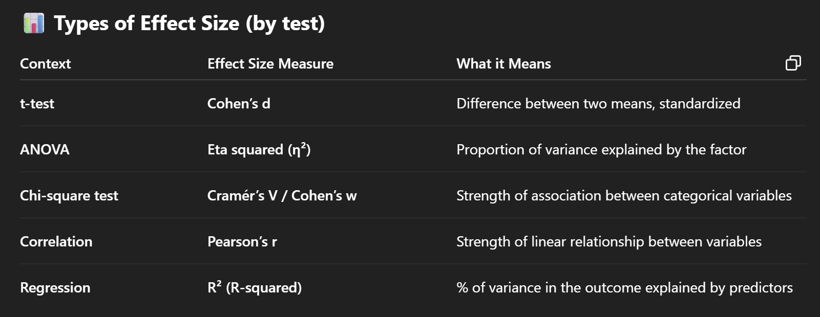
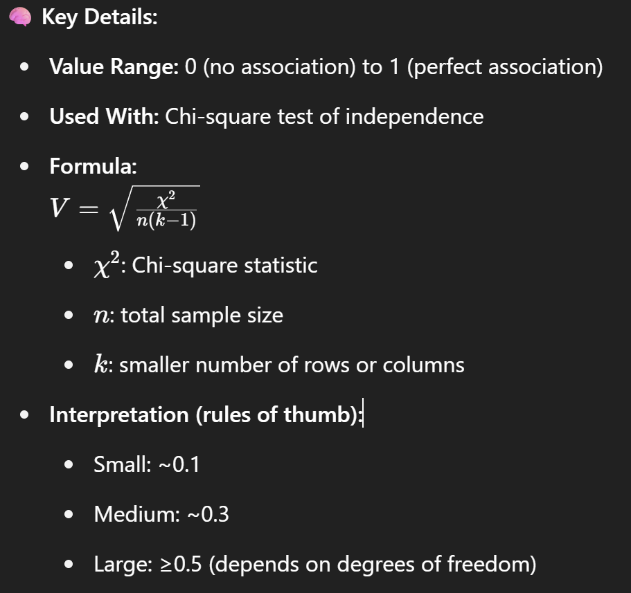
Cramér’s V

Cramér’s V measures the strength of association between two nominal (categorical) variables.

chi-squeare of independence

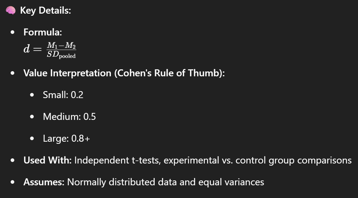
Cohen’s d

Cohen’s d measures the effect size between two means (e.g., in a t-test).

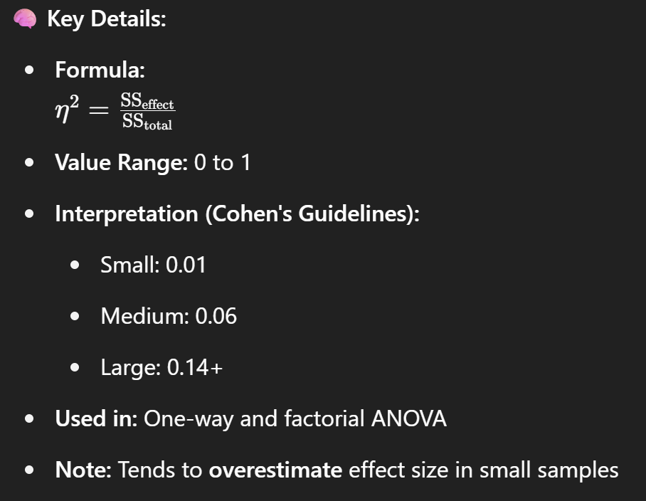
eta squared (η²)

Eta squared (η²) measures the proportion of variance explained by a factor in ANOVA.

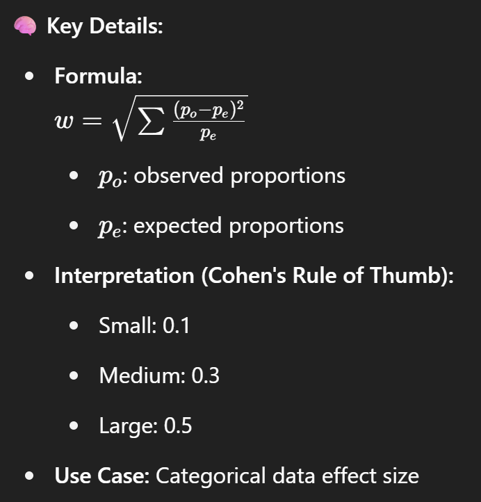
Cohen’s w

Cohen’s w measures the effect size for a chi-square goodness-of-fit or independence test.

Descriptive Statistics

Descriptive statistics refers to the process of summarizing and analyzing data to describe its main features in a clear and meaningful way. It is used to present raw data in a form that makes it easier to understand and interpret.

Inferential Statistics

Inferential statistics involves using data from a sample to make predictions, generalizations, or conclusions about a larger population. Unlike descriptive statistics, which simply summarizes known data, inferential statistics makes inferences or draws conclusions that go beyond the available data.

critical value

A critical value is a threshold in statistical hypothesis testing that helps determine whether to reject the null hypothesis. It marks the boundary between results that are considered statistically significant and those that are not.