Microecomonics I

homo economicus

• is rational (chooses what he thinks is best for him)

• maximises individual utility

  • depends on one’ s own bundle of goods/income

  • free of emotions

  • makes no errors in information processing

Gary Becker on economics

“Economics is the combined assumptions of maximizing behaviour, market equilibrium, and stable preferences, used relentlessly and unflinchingly.”

basic rule of cost-benefit analysis

Realize any action x, as long as B(x) > C(x)

benefit B(x)

Maximum willingness to pay for action x (hypothetical question if x is not sold on the market)

cost C(x)

Cost of action expressed in monetary terms (hypothetical question if x is not sold on the market)

reservation price

Price that makes you indifferent between realizing and not realizing x

What to look out for when making decisions

1. take implicit costs into account

2. ignore sunk costs

3. measure cost and benefit in absolute terms

4. take the difference between average and marginal cost into account

implicit costs

Value of the next best alternative that cannot be realized if you realize x

(“What opportunities am I giving up by choosing x?”)

sunk costs

Historical costs that have already been incurred and are therefore no longer relevant to the decision (sunk cost fallancy)

equilibrium price and quantity

• price-quantity combination in which the market is satisfied

• excess supply and demand are zero

pareto efficiency

allocation, where it is not possible to make an individual better off without making another individual worse off

price cap

• below the equilibrium price: creates excess demand

• above the equilibrium price: no effect

price support

• keeps the price above the equilibrium level

• government is becoming an active buyer in the market

• creates excess supply

functions of prices

• rationing function: consumers recieve the goods they value most

• allocation function: resources are used for the production of goods for which they are most productive

factors shifting the demand curve

• income

• preferences

• prices of substitutes and complements

• expectations

• population size

normal good

quantity demanded increases with an increase in income

inferior good

quantity demanded decreases with an increase in income

factors shifting the supply curve

• technology (cost-reducing)

• factor prices

• number of providers on the market

• expectations

• weather

budget line

• combination of goods that fully exploit the income at given prices

• slope: price ratio = - P_A/P_B

  • indicates opportunity cost for an extra unit of the other good/exchange rate between both goods

composite good

• all other goods, than the one analysed

• often standardized to 1€

assumptions on preference ordering

• completeness

• monotony/non-satisfaction: more is better

• transivitiy

• convexity: mixed bundles are better than extreme bundles

• continuity: small changes in goods only lead to small changes in preferences

indifference curve

combination of all bundles of goods between which an individual is indifferent

characteristics:

• ubiquitous: each bundle is on an indifference curve

• can’t cut each other

• have a decreasing slope, due to convexity

marginal rate of substitution

• quantity of a good that an indiviual is willing to give up to abtain an additional unit of another good, while maintaining the same level of utility

• slope of the indifference curve

price-consumption-curve (PCC)

shows all optimal bundles, that arise from a variation in price (income and other prices remain constant)

income-consumption-curve (ICC)

shows the optimal bundles of two goods consumed for changes in income at given prices

Engel-curve

shows the optimal consumption of one good for changes in income at a given price

substitution effect

• tendency of consumers to replace a more expensive item with a cheaper alternative when its relative price rises

• always negative

income effect

change in demand for a good or service caused by a change in a consumer's purchasing power

total effect of a price change

substitution effect + income effect

Giffen-good

• good for which consumption increases with prices

• inferior good

aggregating demand curves

individual demand curve: P = a - b*Q_i

market demand curve: P = a - (b/n)*Q_i

definition price elasticity of demand

• percentage change in demand for a good when the price of the good changes by one percent

• independent of units

formula price elasticity of demand

ε = (ΔQ/Q)/(ΔP/P)

or

ε = P/Q * 1/slope

inelastic demand

ε > -1

quantity changes underproportionally to a price change

isoelastic demand

ε = -1

quantity changes proportionally to a price change

elastic demand

ε < -1

quantity changes overproportionally to a price change

calculation slope

ΔP/ΔQ

or

coefficient (δP/δQ) in the point

perfectly elastic demand

ε = - ∞

horizontal demand curve

perfectly inelastic demand

ε = 0

vertical demand curve

calculation price elasticity segment ratio method

ε = EC/AC

… = GE/GC * GC/FC = GE/FC

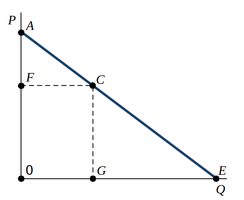
isoelastic demand curve

P = k/Q^1/ε

price elasticity revenue maximization

… if the price elasticity | ε | = 1

price elasticity depends on…

• substitutability: high substitutability → high elasticity

• share in budget: high share → low elasticity

• time: short term → high elasticity, long-term → low elasticity

defintion income elasticity of demand

percentage change in demand for a good when income changes by one percent

formula income elasticity of demand

η = (ΔQ/Q)/(ΔY/Y)

or

η =Y/Q * 1/(slope of Engel-curve)

income elasticities for different types of goods

inferior goods

• 1% increase in income leads to a decrease in demand

• η < 0

necessary goods

• 1% increase in income leads to a <1% increase in demand

• η < 1

luxury goods: η > 1

• 1% increase in income leads to a >1% increase in demand

definition cross price elasticity of demand

change of demand for one good, after change of price for another good

formula cross price elasticity of demand

… for goods X and Z

• ε_xz= (ΔQ_x/Q_x) / (ΔP_z/P_z)

• ε < 0: goods are complements

• ε > 0: goods are substitutes

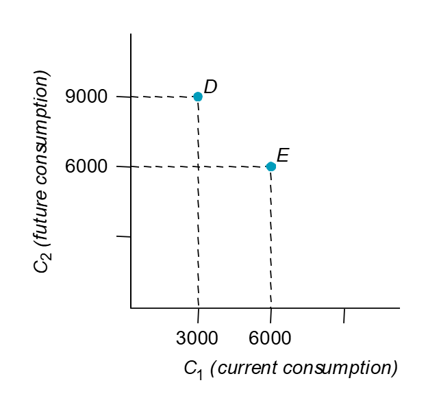
basic question intertemporal decisions

How would a consumer distribute consumption across time?

intertemporal decisions present value

present value of a payment X in T years with interest rate r: X/(1+r)^T

intertemporal decisions present value of lifetime income

= present value of lifetime consumption

M₁ + M₂/(1+r) = C₁ + C₂/(1+r)

defintion and formula intertemporal marginal rate of substitution

• number of consumption of units in the future that an individual would be willing to give up in order to obtain another unit of present consumption, at a constant level of utility

• Δc₂/Δc₁

interpretation IMRS (intertemporal marginal rate of substitution)

IMRS = 1 : consumption can take place today or tomorrow

IMRS > 1 : consumption is valued stronger today

IMRS < 1 : consumption is valued stonger tomorrow

intertemporal decisions effect of reduction in interest rates

income effect:

• borrower has more income → income effect increases present and future consumption

• saver has less income → income effect decreases present and future consumption

substitution effect (trading between present and future consumption)

• saving becomes less attractive → increase in present consumption and decrease in future consumption

permanent income hypthesis (Milton Friedman)

• individuals do not base their consumption decisions on the current income of this period, but on permanent/lifetime income (present value of income over life)

• in each period only a part of the permanent income is consumed

  • increase in income in a period leads to a proportionally smaller increase in consumption in that period (parts of the additional income are used for future consumption)

• practical implication: “consumption smoothing” through loans

intertemporal decisions time preferences

• most people have a present preference or bias

• time preferences differ between people

effect of a price change normal good

substitution effect and income effect reinforce each other

effect of a price change inferior good

substitution effect and income work in opposite directions

income and substitution effect perfect complements

income effect = total effect

substitution effect = 0

income and substitution effect perfect substitutes

income effect = 0

substitution effect = total effect

production function

• Q = F(K, L); K = capital, L = labour

• provides the highest possible output Q for a given combination of production factors

• changes due to technological

production short-run

longest period of time during which the quanitity used cannnot be varied by at least one input factor

production long-run

shortest period of time needed to change the quantities of all input factors used

production variable input

input factor, the amount of which can be adjusted in the short term

production fixed input

input factor whose quantity cannot be adjusted in the short term

shape of the production function

• runs through the origin

• for small factor input quantities, the marginal product of the variable input factor initially increases

• from a certain amount of factor input, the marginal product of the variable factor decreases

law of diminishing returns

If the other input are held constant, the output increases resulting from an increase in the amount of the variable factor and decreases (from a certain point) with the amount of this variable factor

production total product

production quantity as a functino of the quantity of the variable input factor used

production marginal product

change in the quantity of production when an input is increased by one unit

→ derivative

production average product

production quantity per unit of a given input factor

• in each point of the total product curve is the slope of the line through the origin and this point (Q/L)

• intersects with the marginal product at it’s maximum (APL max)

production isoquant

set of all input combinations that result in the same output level

production marginal rate of technical substitution (MRTS)

ratio at which one factor of input production can be exchanged for another without changing the level of output

• for perfect substitutes: 45° angle

• for perfect complements: L-shape

production constant returns to scale

an increase of alll production factors by x-percent increases production by x-percent

production increasing returns to scale

an increase of all production factors by x-percent increases production by more than x-percent

production decreasing returns to scale

an increase of all production factors by x-percent increases production by less than x-percent

Cobb-Douglas production function

Q = mK^α*L^β

Leontief production function

perfectly complementary inputs

Q = min(aK, bL)

costs fixed costs (FC)

costs that are not directly related to the output quantity in the short term (costs of all fixed production factors)

always according to output quantities

costs variable costs (VC)

costs that vary with the output quantity in the short term (costs of all variable production factors)

always according to output quantities

costs total costs

all production costs

TC = FC + VC

always according to output quantities

costs capital costs

implicit rental value of using physical assets, fixed costs

FC = r*K₀; r = interest rate per unit, K₀ = units of capital used

increasing marginal product…

for concave shape of the curve

decreasing marginal product…

for convex shape of the curve

average fixed costs (AFC)

fixed costs divided by the output quantity

approaches zero for infinity

average variable cost (AVC)

variable cost divided by the output quantity

has a global minimum

average total cost (ATC)

total costs divided by the output quantity

has a global minimum

marginal costs (MC)

change in total costs, resulting from a change in output by one unit

→ derivative of the variable costs, fixed costs drop out as they are constant

relation of marginal and average costs

marginal costs curve intersects ATC- and AVC-curve at its minimum

additionally:

• if MC < ATC/AVC: average cost decreases with the output quantity

• if MC > ATC/AVC: average cost increases with the output quantity

costs allocation between two production sites

production quantities should be selected such that the marginal costs at the two production sites are the same

relationship between the MC and MP

minimum of the MC-curve corresponds to the maximum of the MP-curve

MC = w/MP

relationship between the AVC and AP

minimum of the AVC-curve corresponds to the maximum of the AP-curve

AVC = w/AP

isocost line

quantity of all input factor bundles that fully utilize a given production budget at given factor prices

slope: negative factor price ratio (-w/r)

maximising output for given expediture

tangential point between the isoquant and the isocost line

minimum costs for a given output level

tangential point between the isoquant and the isocost line

cost/output maximisation optimum

• MP_L/w = MP_K/r

• consequence: if the last additional euro invested in an input factor generates more additional output than with the last euro invested in the other input factor, more of the first factor should be used

• at cost minimum: ration of marginal product to factor price must be same for all input factors

capital-to-labour-ratio

• varies across countries and companies

• leads to different optima with the same underlying production function

output expansion path

curve of tangential points (minimum cost combinations) resulting from a shift in the isocost line for a given isoquant set

long-term costs (LTC)

• can be presented as a function of output from the output expansion path

• LTC-curve always runs through the origin (company can liquidate inputs)

LTC and returns to scale

• constant returns to scale: constant slope

• increasing returns to scale: concave function

• decreasing returns to scale: convex function

economies of scale

production processes with constant, decreasing or increasing returns to scale are special cases

• returns to scale often vary along the production process