Unit 5 - Density Curves & Normal Distribution

Histogram

A histogram is a graph that shows how the data is spread out. This can be thought of as a photograph of the actual data. Suppose the scores are grouped like this:

Score Range	Number of Students
40–49	5
50–59	10
60–69	25
70–79	35
80–89	20
90–99	5

• The horizontal axis (x-axis) shows the score ranges.

• The vertical axis (y-axis) shows how many students are in each range.

• Each bar touches the next bar because scores are continuous data.

Purpose of Histograms

Histograms can take the shape of symmetric (bell shaped), right skewed (positively skewed), left skewed (negatively skewed), uniformed, bimodal, multimodal or outliers.

A histogram helps you see information like:

• Where most data values fall

• How spread out the data is

• Whether there are unusual values (outliers)

• The overall shape of the distribution (e.g. symmetric, right skewed, left skewed, etc).

For example, if the tallest bar is 70-79, then most students scored in that range.

Pros and Cons of Histograms

A histogram is a graph showing the distribution of numerical data by grouping values into intervals (called bins).

Pros:

• Helps identify whether data is symmetric, skewed or has multiple peaks.

• Displays where most values are concentrated.

• Can highlight gaps, clusters and outliers.

• Makes thousands of data points easier to understand at a glance.

• Multiple histograms can be used to compare datasets.

Cons:

• Different bin sizes can make the data look different

• Exact values are not shown

• Not ideal for small datasets

• Can hide important details

• Less useful for categorical data

Density Curves

A density curve helps us focus on the overall pattern of the data. It is a smooth theoretical model of data distribution, whereas histograms are the actual graphed data. A proportion is the area under a density curve that represents a proportion (or probability).

There are two key parts to a density curve. This includes:

1. It is always on or above the horizontal x axis.

   • It can only be positive or zero.

   • It cannot go below zero.

2. The total area under the curve equals 1 (this represents 100% of the probability / observations). Total area under 1 = 100% of the area.

   • This concept leads directly to proportions.

Proportion

A proportion is a part of a whole (percent). It tells us what fraction of the group has a particular characteristic.

Proportion = The Number in the Group / divided by the total number

• Suppose 25 / 100 students scored between 80 and 89.

• Proportion would be 25 divided by 100 = 0.25

This means:

• Proportion = 0.25

• Percentage = 25%

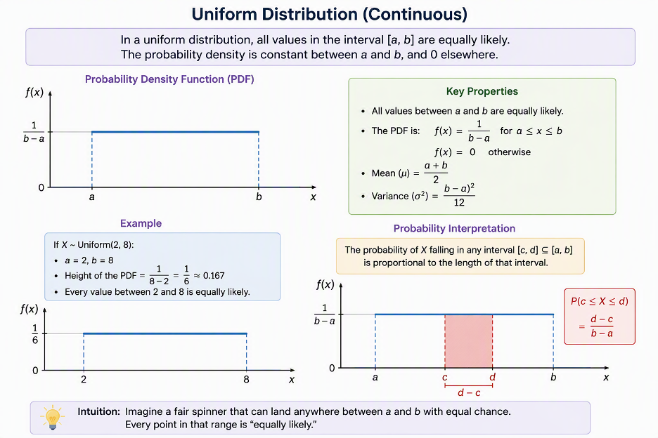
Uniform Distribution

A distribution where all values within a given range are equally likely to occur. Uniform means that there is an equal chance that it could occur everywhere.

• Every value has the same chance of occurring.

• No part of the distribution is more likely than another.

• The probability is spread evenly across the range.

• The density curve is a flat horizontal line.

Examples of where uniform distribution is used:

• Rolling a fair die.

  • Each number has the same chance of occurring. This is a discrete uniform.

• Drawing a random card from a shuffled deck.

  • Every card has an equal chance of being selected.

• Random arrival times.

  • If a bus can arrive anytime between 1:00 p.m. and 2:00 p.m. with equal likelihood, the time follows a continuous uniform distribution.

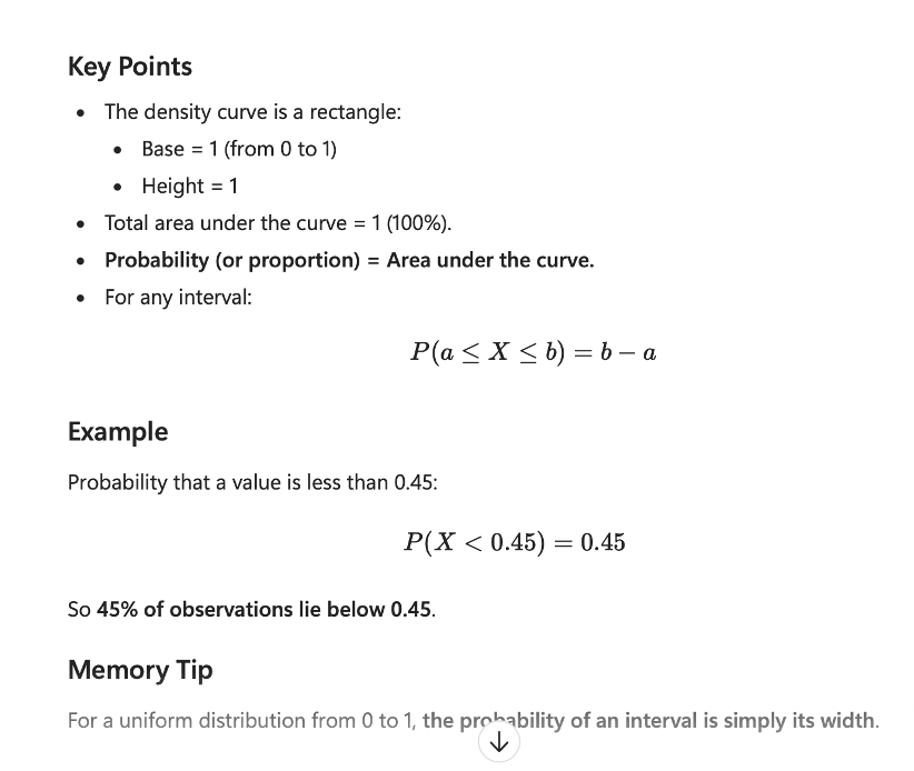
What is a Uniform Distribution from 0 to 1?

From 0 - 1 every value is equally likely to occur.

• The density curve is a flat rectangle:

  • Base = 1 (from 0 to 1)

  • Height = 1

• For a uniform distribution from 0 to 1, the probability of an interval is the length of the interval.

  • Probability = Upper level value - lower value (which is just the width of an interval)

  • Wide intervals = larger probabilities

  • Narrower intervals = smaller probabilities

• Example: Imagine a bus could arrive anytime between 0 - 10 minutes, and every minute is equally likely. What is the probability that the bus arrives between 2 - 5 minutes?

  • Find the width of the interval: 5 - 2 = 3. Interval has a width of 3 minutes.

  • Divide the number by the total width 3 / 10 =0.3 0.30 or 30%.

What is the proportion of observations that lie below 0.45?

• Hint: What is the area of a rectangle?

• The area of a rectangle is base * height = (0.45)(1) = 0.45

Key Density Curve Rule: In a density curve, the proportion of observations = the total area under the curve.

Step 1: Identify the shape

For a uniform distribution from 0 to 1, the density curve is a rectangle with:

• Base = 1 (from 0 to 1)

• Height = 1

Step 2: Find the area below 0.45

The shaded region goes from 0 to 0.45. So the rectangle has:

• Base = 0.45

• Height = 1

Step 3: Use the area of the rectangle formula

• Area = Base x Height

• Area = 0.45 × 1

• Area = 0.45

Step 4: Interpret the answer

Because area = Proportion: P(X < 0.45) = 0.45

So the proportion of observations below 0.45 is 0.45. 45% of observations lie below 0.45.

What Different Density Shapes Are There?

The shape of the distribution: The overall appearance of the curve shows the distribution’s shape. Density curves can come in many different shapes.

Common shapes include:

• Bell-shaped (normal): Most values are near the center. Fewer values are at the extremes. Symmetric.

• Uniform (all values equally likely): Looks flat. Values occur about equally often across the range. No obvious peak.

• Skewed (Left or Right): One tail is often longer than the other.

  • Left Skewed: Tail stretches to the left, so most data is on the right. There area a few low values that pull the tail to the left. Mean < Median.

  • Right Skewed: Most data is on the right. A few large values pull the tail right. Mean > Median.

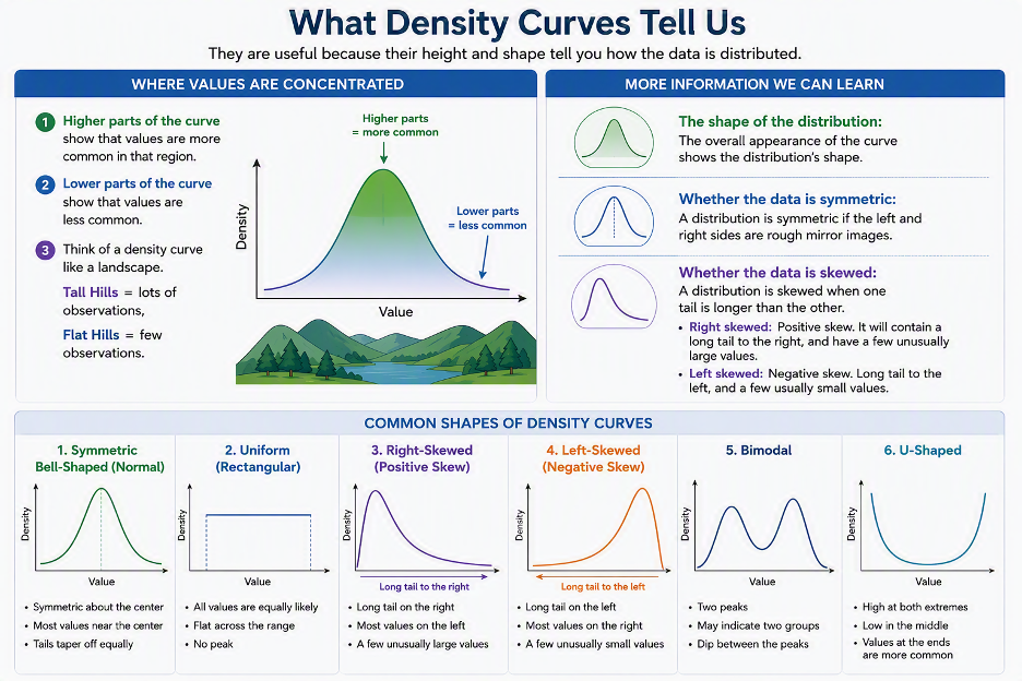
What Does a Density Curve Show?

They are useful because their height and shape tell you how the data is distributed. It also shows:

Where values are concentrated:

1. Higher parts of the curve show that values are more common in that region.

2. Lower parts of the curve show that values are less common.

   • Think of a density curve like a landscape. Tall Hills = lots of observations, Flat Hills = few observations.

The shape of the distribution: The overall appearance of the curve shows the distribution’s shape.

Whether the data is symmetric: A distribution is symmetric if the left and right sides are rough mirror images.

Whether the data is skewed: A distribution is skewed when one tail is longer than the other.

• Right skewed: Positive skew. It will contain a long tail to the right, and have a few unusually large values.

• Left skewed: Negative skew. Long tail to the left, and a few usually small values.

What Two Conditions Must be Met for Every Density Curve?

Two conditions are required because a density curve represents probabilities, and probabilities have certain rules. For every density curve in statistics, these two conditions must be true:

1. The total area under the curve equals 1

   • This represents the fact that the total probability of all possible outcomes is 100% (or 1).

   • Part of the curve would mean part of the probability.

   • Area under a density curve represents the probability.

2. The curve is never below the horizontal axis

   • A density curve cannot have negative values because probabilities cannot be negative.

What Does Distribution Mean?

Think of looking at patterns of how all the data is spread out. It shows which values occur the most often in data, which occur less often, and the overall pattern of the data.

For example:

• Think of it as we have test scores: 60, 65, 70, 70, 72, 75, 78, 80, 95, 90.

• Dataset: This is the actual list of scores. The actual numbers.

• Distribution: This is the pattern you see when you look at those scores as a group. Overall pattern of those numbers.

  • Most scores are around 70 - 80.

  • Very few scores are at the low and high ends.

  • The shape is roughly a bell shape.

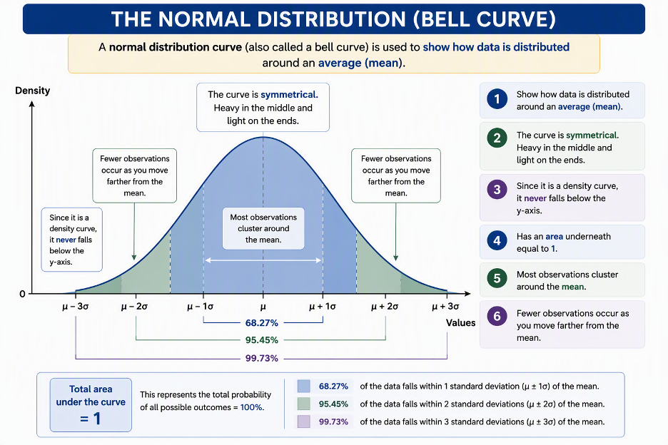
Traits of a Normal Distribution Curve

A normal distribution curve (also called a bell curve) is used to:

• Show how data is distributed around an average (mean).

• The curve is symmetrical. Heavy in the middle and light on the ends.

• Since it is a density curve, it never falls below the y-axis.

• Has an area underneath equal to 1.

• Most observations cluster around the mean.

• Fewer observations occur as you move farther from the mean.

The 68-95-99.7 Rule for ND

This rule only applies to a normal bell-shaped distributionand tells you how much of the data falls within certain numbers of standard deviations from the mean.

About 68% of values (people) fall within 1 standard deviation of the mean. For example about 68% of the scores fall within that range.

• Mean ± 1σ: 68%

• Mean to 1σ: 34%

About 95% of people fall within 2 standard deviations of the mean. For example about 95% of scores fall within that range.

• Mean ± 2σ: 95%

• 1σ to 2σ: 13.5%

About 99.7% of people fall within 3 standard deviations of the mean. For example about 99.7% of scores fall within that range.

• Mean ± 3σ: 99.7%

• 2σ to 3σ: 2.35%

• Beyond 3σ: 0.15%

Two Parameters of the Normal Distribution Curve

The normal distribution curve is characterized by two parameters.

This includes the:

1. Population Mean (μ)

   • The average value of the population.

   • Determines the center of the distribution.

   • Moving μ left or right shifts the entire curve.

2. Population Standard Deviation (σ)

   • Measures how spread out the data are.

   • Determines the width of the distribution.

   • A larger σ gives a wider, flatter curve; a smaller σ gives a narrower, taller curve.

Quick way to remember:

• μ (mean): Where the center is

• σ (standard deviation): How spread out the data are

Together, μ and σ completely describe a normal distribution.

Parameter

A characteristic of the whole population that you are interested in studying. The entire population of something.

Examples:

• Parameter: The average age of all University of Manitoba students.

• Parameter: The proportion of all Canadians who support a policy.

• Parameter: The average height of all Manitoba women.

What is a Statistic?

A characteristic calculated from a sample and used to estimate a population parameter. Something calculated from a sample.

Example: Suppose there are 10,000 students at a university (the population). Instead of measuring all 10,000 students, you randomly select 100 students (a sample).

If the average height of those 100 students is 172 cm, then:

• 172 cm is a statistic (sample mean, x̄).

• The average height of all 10,000 students would be a parameter (population mean, μ).

What Two Statistics Correspond to Two Parameters?

The two parameters of the population mean, and the population standard deviation correspond to the sample mean, and the sample standard deviation.

• These are the sample versions of the population mean and population standard deviation.

Population	Sample
Population mean = μ	Sample mean = x̄
Population standard deviation = σ	Sample standard deviation = s

How Does the Mean and Standard Deviation Describe the Normal Distribution?

Population Mean μ is the measure of centre of the normal distribution. It can take any positive or negative value.

• Examples include temperatures, test scores, income, weights or heights.

• Can be left (-) or right (+) on the number line.

Population Standard Deviation σ is the measure of spread / variability of the normal distribution. Its values cannot be negative, however it can be 0.

• Average distance from the center.

• Examples include spread of test scores, variation in salaries, variability in temperatures.

What does X ∼ N (μ,σ) mean?

"X follows a normal distribution with mean μ and standard deviation σ."

X is normally distributed with the:

• μ: Population mean (center of the curve)

• σ: Population standard deviation (spread of the curve)

Example:

X ∼ N (100,10). X is normally distributed with the mean of 100, and a standard deviation of 10.

What Does Normally Distributed Mean

When data is normally distributed, it forms a bell-shaped curve.

N = normal distribution, however, sometimes questions will just outright say “normally distributed"

AND the question will always appear in the formula of:

X ∼ N (μ,σ)

• Most values are near the average (mean).

• Fewer values are far from the average.

• The distribution is balanced and symmetrical.

Suppose we have a variable for which a normal density model is appropriate. It is known that (μ) = 150, and (σ) = 20.

What proportion of our observations fall between 130 and 170?

Note that 130 is 20 less than (1 standard deviation below) the mean of 150. Similarly, 170 is 1 standard deviation above the mean.

Mean: 150

Standard Deviation: 20

How far are the endpoints from the mean?

• For 130: 150 − 130 = 20

• For 170: 170 − 150 = 20

Both are exactly 1 standard deviation away because one SD = 20.

Which rule matches 1 standard deviation?

• 68%

If the:

• Mean (μ) = 200

• Standard Deviation (σ) = 10

What proportion falls between 180 and 220?

1: Find the center. The mean is 200, which is located right at the center.

2: Find how far 180 is from 200. 200 - 180 = 20.

3: Find how far 220 is from 200. 220 - 200 = 20.

• So now we know that both 180 and 220, have a distance of 20 between them.

4: How big is one standard deviation. The question tells us that Standard Deviation (σ) = 10. So 1 standard deviation = 10.

5: Compare the distance with the standard deviation.

• 180 is 20 away from 200

• 220 is 20 away from 200

And we know:

• 1 SD = 10

• 2 SD = 20

Since the distance is 20: The interval is 2 standard deviations from the mean.

Step 6: To determine which distance it is away do the Distance from the Mean divided by the Standard Deviation (provided) and it will give you 1, 2, or 3.

• For example 20 divided by 10 = 2 SD.

Suppose that we have a variable for which a normal density model is appropriate. It is known that Mean: μ = 150 and σ = 20.

99.7 % of our observations lie between which values?

Identify the percentage. From the rule:

• 68% → ±1 SD

• 95% → ±2 SD

• 99.7% → ±3 SD. So we need 3 standard deviations.

Calculate the 3 standard deviations (because there is 99.7%).

• 1 = 20, so three would be 3 × 20 = 60. 3 SD = 60.

Subtract from the Mean: 150 - 60 = 90 (lower value).

Add to the mean: 150 + 60 = 210 (upper value).

Final Answer: 90 - 210. About 99.7% of observations lie between 90 and 210.

If we are told that the population μ is 150, and that 95% of our data falls between 110 and 190. What is the standard deviation σ equal to?

1 What does 95% mean. So right away we can see that 110 and 190 are 2 SD away from the mean.

• 68% = ±1σ

• 95% = ±2σ

• 99.7% = ±3σ

2 Find the distance from the mean.

• The mean is 150. How far is 110 from 150?

• 150 - 110 = 40.

• How far is 190 from 150?

• 190 - 150 = 40. So the endpoints are each 40 units away from the mean.

3 Connect the distance to standard deviations

• We know that 40 units = 2 standard deviations (2σ=40)

• Divide both sides by 2: σ 40/2. Both sides are divided by 2, because that the the SD number that we are using.

• So σ = 20.

Step 6: To determine which distance it is awa

Distance from the Mean / divided by the Standard Deviatio(provided).

• 40 divided by 2 = 20.

Why Does the Surface Underneath a Density Bell Curve Have to = 1

Dartboard or Pizza Examples

Imagine a Dartboard

• Suppose you throw a dart.

• The dart can land anywhere on the board.

• Since it has to land somewhere, the chance of it landing somewhere on the board is:

• 100% = 1.0

• That's the same idea as the bell curve.

• The bell curve shows all possible outcomes.

Since an outcome must be somewhere on the curve, the total probability under the entire curve is: 1 = 100%

Think of the Curve as a Pizza

Imagine the whole area under the curve is a pizza. The entire pizza = 100% of possible outcomes.

• Left half of the pizza = some percentage

• Middle slice = some percentage

• Right slice = some percentage

All slices together must equal: 100% or 1.0.

Purpose of Standard Deviations Example

The "Crowd at a Concert" Analogy

Imagine everyone in a city lines up by test score.

The average person stands in the middle.

• Within 1 standard deviation: the big crowd around the middle.

• Within 2 standard deviations: almost everyone.

• Within 3 standard deviations: basically everybody.

That's why statisticians remember:

• 68% are within ±1 SD

• 95% are within ±2 SD

• 99.7% are within ±3 SD

Why Do We Care About the Z Score?

The z-score is just tells us How many standard deviations away from the average is this result?

So when you see:

• z = 0.5: Pretty normal

• z = 1.0: Still normal

• z = 2.0: Uncommon

• z = 3.0: Very rare

• z = 4.0: Extremely rare

The bigger the absolute value of z, the more unusual the result.

Z-Score	Meaning
0	Average
±1	A little different from average
±2	Uncommon
±3	Very rare
±4+	Extremely rare

If someone tells you a result has z = 2.25, you can immediately think That’s more than 2 standard deviations above average so it’s pretty unusual.

Exam Scores Scenario

A school exam has:

• Mean (average) score = 70

• Standard deviation = 10

If the exam scores follow a normal distribution, approximately what percentage of students scored:

• Between 60 and 80?

• Between 50 and 90?

• Between 40 and 100?

First, identify how many standard deviations each range is from the mean (70):

Show more lines

• 60 to 80 = Mean ± 1σ → 68%

• 50 to 90 = Mean ± 2σ → 95%

• 40 to 100 = Mean ± 3σ → 99.7%

Most students are within 1 SD, almost all students are within 2 SDs, and virtually everyone is within 3 SDs.

Now say we want to know what percentage of our data falls between 150 and 196 when µ= 150 and σ = 20.

We cannot use the 68-95-99.7% rule because the value 196 is not exactly 1, 2, or 3 standard deviations above the mean. We need another method to find any other area under the normal curve that is not covered by the 68-95-99.7% rule.

The Standard Normal:

• This curve has µ= 0 and σ = 1.

• The area under this curve = 1.

When to Use the Standard Normal Table

This is used where the area of proportion of observations can be from Infiniti to some value of z (which can be found in the z table as a z score). Table entry for z is the areas under the standard normal curve to the left of z.

Use the z-table when the z-score is something like:

• 0.43

• 1.27

• -0.85

• 2.14

These types of numbers are not covered by the 68-95-99.7% rule.

Find the proportion below z = 1.27. Look up 1.27 in the z-table.

You get approximately: P(Z<1.27) = 0.8980. This means that 89.80% of observations are to the left of the z = 1.27.

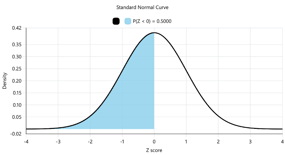
What does this Image Mean?

• The bell curve represents all possible Z-scores.

• The red dashed line marks Z = 0, the exact center of the distribution.

• The blue shaded area is everything to the left of 0.

• Because the standard normal distribution is perfectly symmetric, that shaded region is exactly half of the total area under the curve.

Therefore: P (Z < 0) = 0.5000

This means:

• 50% of the values are below 0.

• 50% of the values are above 0.

• The entire area under the curve equals 1.0000 (100%).

A quick memory trick: Z = 0 is the middle of the bell curve, so the area on either side is always 0.5000.

What Does This Image Mean?

The z-scores only give us an area of the left. To find the right of a z-score we must:

Step 1: Find the area to the left of 1.25

• From the Z-table: P (Z ≤ 1.25) = 0.8944

• This means 89.44% of the area is to the left of Z=1.25

Step 2: Use the fact that the total area is 1

• The entire area under the normal curve is always 1.0000

• So the area to the right of 1.25 is

• P (Z>1.25) = 1 − P (Z≤1.25) = 1 − 0.8944 = 0.1056

So only 10.56% of all values lie above a Z-score of 1.25.

• Left area? Read it directly from the Z-table.

• Right area? Use: Right Area = 1 − Left Area

Z-Table Example (Left Side)

Left Side: "How many people are below this employee?"

Imagine you're a warehouse supervisor.

• Average employee picks 100 orders per day.

• One employee's productivity converts to a z-score of 1.27.

The Z-table tells you: P (Z < 1.27) = 0.8980.

• This means that 89.9% of employees pick fewer orders than this employee.

• So the left side answers What percentage of people are below this person?

  • That is why the Z-table gives the left area.

Z-Table Real World Example Right Side

Right Side: "How many people are above this employee?"

Now your manager asks: What percentage of employees perform better than this employee?

The Z-table already told us: P (Z<1.27) = 0.8980

Since everyone must be either below or above:

• P (Z>1.27) = 1 − 0.8980 = 0.1020. This means that only 10.2% of employees perform better than this employee.

• The shaded right side represents the top performers above this employee.

What does P(Z<−0.93) mean?

For this specific Z-table shown in your screenshot, use it when the question asks for the area (probability) to the LEFT of a z-score.

Use this table when the question asks for a standard normal curve to the left.

Example: Find the area to the left of z = −0.93 on the normal curve.

• Look up -0.93 in the Z-table.

• P(Z<−0.93) = 0.1762

• This means 17.62% of observations are below -0.93.

When do I use P(Z = a) = 0

Also known as P(Z = 2) = 0

Use this rule whenever the question asks for the probability of one exact value in a normal distribution.

The normal distribution is a continuous curve. Probability comes from area under the curve. A single point has no area under the curve, so its probability is always 0.

A single point has:

• no width

• no area

Therefore the probability = 0.

For example:

• P (Z = 2)

• P (Z = −1.5)

• P (X = 100)

The answer is always 0

• P(Z = 2)

• P(Z < 2)

• P(1 < Z < 2)

• P(Z > 2)

• P(Z = 2) → 0

• P(Z < 2)→ Use Z-table

• P(1 < Z < 2)→ Use Z-table

• P(Z > 2) → Use Z-table and subtract from 1

• < : This means left. Less than.

• > : This means right. Greater than.

How to Find the Area Between Two Z-Scores

P(−1.33 ≤ Z ≤ 2.16)

This means what percentage of observations fall between -1.33 and 2.16?

We can’t look this up directly on the z-score because the Z-table only gives P(Z < z), which means the area to the left of a z-score. The table does not give the area between two values. So we need to do a subtraction.

Steps to Find the Area Between Two Z Scores

For example P(−1.33 ≤ Z ≤ 2.16)

Step 1: Find the Area Left of the Larger Z-Score

• Look up 2.16 in the Z-table: P(Z < 2.16) = 0.9846

Step 2: Find the Area Left of the Smaller Z-Score

• Look up -1.33: P(Z < −1.33) = 0.0918

Step 3: Subtract

• The large area includes the small area, so remove it: P(−1.33 ≤ Z ≤ 2.16) = 0.9846 − 0.0918 = 0.8928

What Does 0.8928 Mean?

• 0.8928 = 89.28%. This means that 89.28% of observations are between -1.33 and 2.16

What is the proportion of our data falling between when:

• x = 150

• x = 196

• P(150 < X < 196)

Finding the Answer for Two Z Scores

Because there are two different x values, they must both be calculated (150 and 196) because the question is asking for the probability between two x-values:

P(150 < X < 196)

When you want the area (probability) between two points on a normal distribution, you must convert both endpoints into z-scores.

Step 1: Convert each x-value

• Mean μ=150

• Standard deviation σ=20

• For x = 150: z = 150 - 150 / divided by 20 = 0

• For x = 196: z = 196 - 150 / divided by 20 = 2.30

  • Make sure that when you put it in the calc you click = before dividing.

Step 2: Rewrite the Formula

• So P(150 < X < 196) becomes P(0 < Z < 2.30). This can be read as what area is under the curve between z = 0 and z - 2.30?

Step 3: Look up 2.30 in Z table (full length table)

• P(Z < 2.30) = 0.9893. This means that 98.93% of the curve is the the left of 2.30.

Step 4: Remove the area left of 0.

• P(Z < 0) = 0.5000.

• Subtract 0.9893 - 0.5000 =0.4893

• P(150 < X < 196) = 0.4893 = 48.93%

Z∼N (0,1)

This means that Z follows a normal distribution with mean 0 and standard deviation 1.

Let's break it down:

• Z = the variable (the z-scores)

• ∼ = "is distributed as" or "follows"

• N = Normal distribution

• 0 = mean (μ)

• 1 = standard deviation (σ)

Z-Score Cheat Sheet

Less than (<): P(X < 196). Find the Z score and look it up in the table.

• P(Z < 2.30) = 0.9893.

• Answer = table value.

Greater than (>): P(X > 196). Find the z-score and subtract from 1.

• 1 - P(Z < 2.30).

• 1 - 0.9893 = 0.0107

• Great than = 1 - table value

Between two values: P(150 < X < 196). Find both z-scores.

• P(0 < Z < 2.30).

• Then P(Z < 2.30) - P(Z < 0).

• 0.9893 - 0.5000 =0.4893.

• Between = Larger table value - smaller table value.

Left of mean: P(X < 150).

• Since the mean is 150.

• Z = 0 is equal to 0.5000 is the Z chart (50%).

• P(Z < 0) = 0.5000 or 50%

• Always equates to half or 50%.

Right of the mean:

• P(X > 150)

• 1 - 0.5000 = 0.50 or 50%

Tricks for When an Answer Will be a Negative

Trick #1: Compare the area to 0.5

If you're working with a left-tail probability P(Z<z)

• If the area is less than 0.5 → z is negative

• If the area is greater than 0.5 → z is positive

• If the area is exactly 0.5 → z is 0

• P(Z < 0.0495) must be negative.

Trick #2: Picture the bell curve

• The center of the curve is z = 0.

• If there is only a tiny amount of area left, the cutoff point must be far to the left. Therefore, negative.

Trick #3: If the question says "95% are greater than..."

• P(X > 25) = 0.9595. This means that 25 is way over on the left side of the distribution. This is because almost everything is greater than 25.

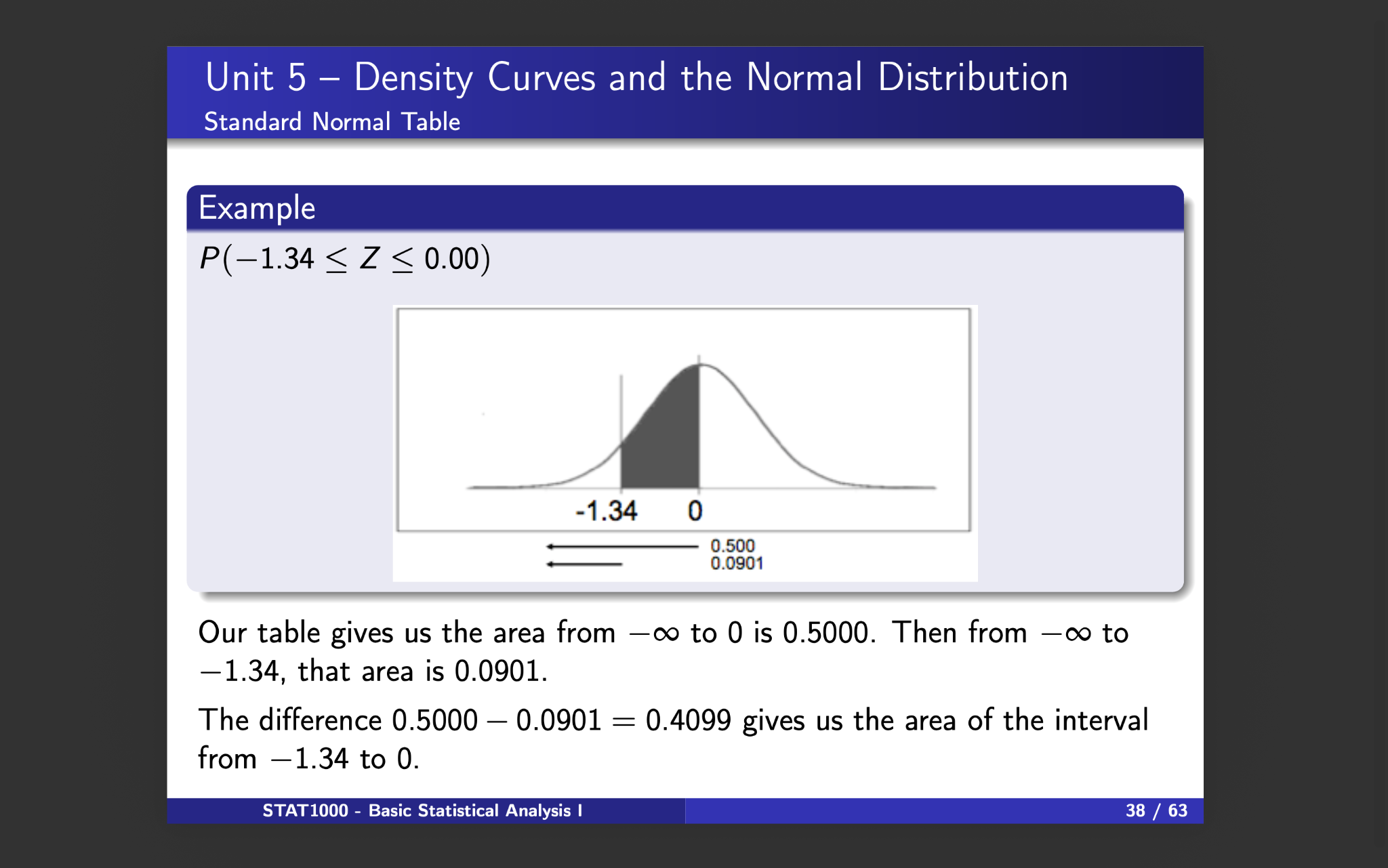
What does P(−1.34 ≤ Z ≤ 0) mean?

This is asking what is the probability that a Z-score falls between -1.34 and 0? On the bell curve, that's the shaded area between z = -1.34 and z = 0.

Step 1: Understand the normal curve

The normal distribution is perfectly symmetrical.

• Half the area is on the left of 0 = 0.5000

• Half the area is on the right of 0 = 0.5000

Since probabilities are represented by area under the curve, the area from −∞ to 0 is always 0.5000.

Step 2: Look up -1.34 in the Z-table

• The Z-table tells us: P(Z ≤ − 1.34) = 0.0901

• This means the area from −∞ to −1.34 is 0.0901.

Step 3: Subtract to get the shaded area

• We want only the area between −1.34 and 0.

• This means that P(−1.34 ≤ Z ≤ 0) = 0.4099. So there is about a 40.99% chance that a standard normal random variable falls between −1.34 and 0.

Tip for Questions with Two Z Scores

Whenever you're asked for the probability between two z-scores, think:

Area between = larger cumulative area - smaller cumulative area

That's exactly what they did here:

• 0.5000 − 0.0901 = 0.40990

• The shaded region on the graph is the probability you're looking for.

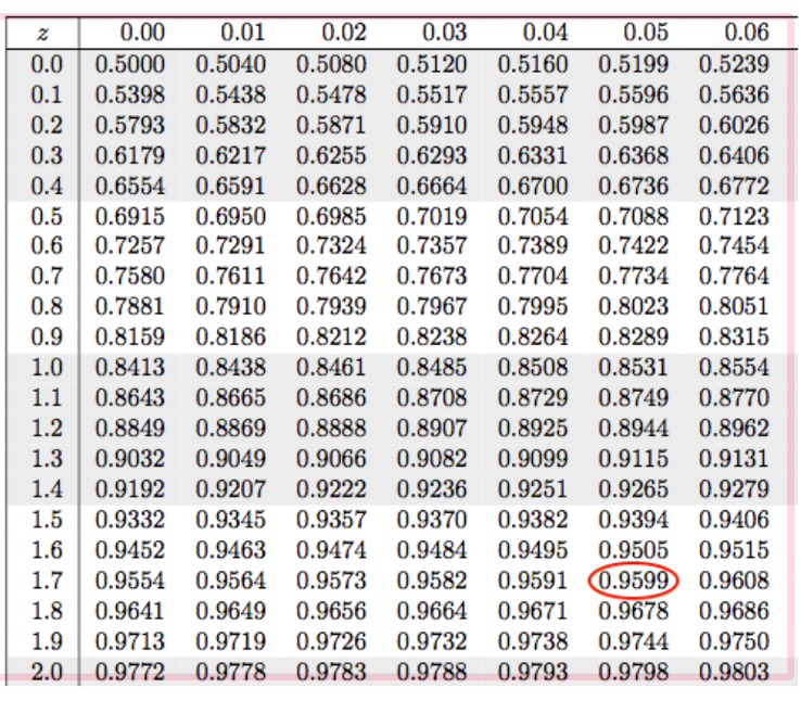
Z-Table

A chart used in statistics to find probabilities associated with a z-score. The side and top part of this chart will tell you how far in standard deviations the mean is from the value (Row: 2.1, and Column 0.07 means 2.17). This value corresponds to 0.9850 or 95.80%.

The Z table helps you answer questions like:

• What percentage of values are below a certain point?

• How many standard deviations away from the mean am I?

• What percentage of data lies there or below?

• What percentage are above a certain point?

• How unusual is a particular observation?

• What probability corresponds to a z-score?

Z Score Question

P(Z > z) = 0.1170

Step 1: Convert to a left-side probability

• Your Z-table gives areas to the LEFT, not the right.

• Since the whole curve equals 1.0000: 1.0000 − 0.1170 = 0.8830

• Now we know that P (Z < z) = 0.8830. 88.30% of the curve is to the left of z.

Step 2: Find 0.8830 inside the Z-table

Now you're working backwards. Instead of starting with z and finding an area. Search the body of the table for 0.8830. You'll find a value very close to it at 0.88298.

• Row: 1.1

• Column: 0.09

• This gives you the z score of 1.19

• Z = 1.19

Density Curve Question Type Cheat Sheet

Less Than (<):

• Complete the question using the z formula.

• Then find the z-score in the table value.

• This is asking for the area to the left of the z-score (which is what the z-table mainly provides us with).

Greater Than (>):

• Use the z formula to find the value.

• Then subtract 1 from the Z score table value that you find (1 - Z score table value).

• This is asking us for the area of the right of the z score, which is why we need to subtract 1.

Between P(X < x) =:

• Take both numbers provided and change them with the Z formula.

• Subtract the bigger # from the smaller number.

• Find the Z score once both are subtracted.

Bottom %: This will be a negative Z score.

Top %: This will be a positive Z score.

Question Types

Find a probability P(X > 1125):

• Key words: Probability, what %, what proportion, chance that, how many above or below.

  • Change the value to a z score using formula.

  • Use the z-table to find the z-score.

  • Answer is probability found in the z score.

Find a cutoff score (Find x):

• Key words: Find the score, find the mark, find the temp, find the passing grade, what value x.

• Calculate using the z score formula.

• Calculate with x = u + z(o).

• The answer you get is the x.

Bottom %:

• Key words: Lowest 10%, failed, poor performers, worst %.

• This will be a negative z score.

Top %:

• Top will be positive number.

• Key words: Top 5%, highest 10%, best students, elite performers.

• Subtract 1 from %.

• 1 - 0.05 =0.95 0.9500

• Z score = 1.645

Question Type Key Word Recognition

1. Less than: Less than, shorter than,

2. Greater than: More than,

3. Between: What proportion is between, between 150 pounds and 170 pounds, from ____ to ______, lies within, falls between

4. Bottom %: Bottom %,

5. Top %: Top % of students,

Less Than < (Table Value)

Steps to Answer a Less Than Question

• Complete the question using the z formula given.

• Once the equation is complete, find the value in the z-table.

  • The value will be the Z-score on the column side / top.

• Find the value in the table body.

• Less than is asking for the left area of the z-score. P(Z < z)

• Can use the z-table amount directly as it already gives you what you need.

  • Must add up to 1 or 100%.