Week 3 and 4: Segmentation

Goal of grouping in vision

Group features that belong together

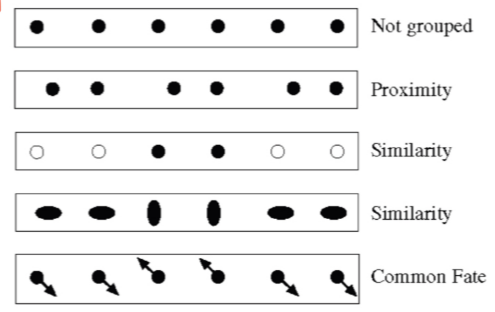
Gestalt psychology

Human visual system tends to group things together

Top-down segmentation

Pixels belong together because they are from the same object

Bottom-up segmentation

Pixels belong together because they look ‘similar’

K-means clustering algorithm

1. Randomly initialise the cluster centers c_1, \ldots, c_K

2. Given cluster centers, determine points in each cluster

   1. For each point p, find closest c_i. Put p into cluster i

3. Given points in each cluster, solve for c_i

   1. Set c_i to be mean of points in cluster i

      1. If c_i have changed, repeat step 2

Properties of k-means

Will always converge to some solution

Can be a local minimum: does not always find the global minimum of objective function

Feature space

E.g. intensity (1D), colour (3D)

Why is feature space important

Encodes whatever property is desirable
E.g. for spatial coherence, cluster in 5D instead to encode similarity and proximity

Pros of k-means

• Simple, fast to compute

• Converges to local minimum within-cluster squared error

Cons of k-means

• Setting k

• Sensitive to initial clusters

• Sensitive to outliers

• Detects spherical clusters only

Multivariate normal distribution notation

\mathcal{N}(\mathbf{x}; \mathbf{\mu}, \Sigma) where mu is a vector containing mean position and sigma is a symmetric “positive definite” covariance matrix

Probabilistic clustering basic idea

Instead of treating the data as a bunch of points, assume they are all generated by sampling a continuous function

Function is called a generative model, defined by a vector of parameters \theta

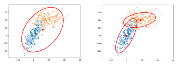
Why use Mixture of Gaussians model

Single normal distribution is often not good enough to cluster multiple groups

Expectation Maximisation (EM) algorithm goal

Find blob parameters \theta that maximise the likelihood function P(data|\theta)

Expectation Maximisation (EM) algorithm approach

1. E-step: Given current guess of blobs, compute ownership of each point

2. M-step: Given ownership probabilities, update blobs to maximise likelihood functionl

3. Repeat until convergence

Expectation Maximisation (EM) algorithm details

1. E-step: Compute probability that point x is in blob b, given current guess of \theta

   1. M-step: Compute probability that blob b is selected, the mean of blob b and the covariance of blob b

Applications of EM

• Any clustering problem

• Any model estimation problem

• Missing data problems

• Finding outliers

• Segmentation problems

Pros of Mixture of Gaussians, EM

• Probabilistic interpretation

• Soft assignments between data points and clusters (vs hard assignments in K-means)

• Generative model, can predict novel data points

• Relatively compact storage

Cons of Mixture of Gaussians, EM

• Local minima

• Initialisation

• Need to know number of groups

• Need to choose generative model

• Numeric problems are a nuisance

What is often a good idea during initialisation of Mixture of Gaussians EM

Good idea to start with some k-means iterations so it’s not completely random

Mean-shift algorithm

1. Initialise random seed, and window W

2. Calculate center of gravity (“mean”) of W

3. Shift the search window to the “mean”

   1. Repeat 2 until convergence

Real Modality Analysis

Can start the mean-shift algorithm from multiple points and parallelise the process.

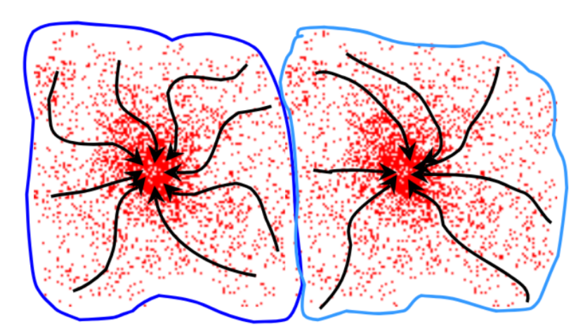
Mean-shift as used for clustering

Cluster becomes all the data points in the attraction basin of a mode, where the attraction basin is the region for which all trajectories lead to the same node

Pros of mean-shift

• General, application-independent tool

• Model-free, does not assume any prior shape on data clusters

• Single parameter (window size h)

• Finds variable number of modes

  • Robust to outliers

Cons of mean-shift

• Output depends on window size

• Window size selection is non-trivial

• Computationally expensive (~2s / image)

  • Does not scale well with dimension of feature space (unviable beyond 3D)

Good news with mean shift window size selection

If we do select the right window size, it will find a global solution

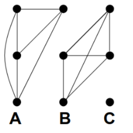
How to represent an image as a graph

• Fully connected graph

• Node for each pixel

• Edge between every pair of pixels (p,q)

• Affinity weight for each edge w_{pq} which measures similarity

Idea of graph-based segmentation

Break the graph into segments by deleting edges that cross between segments.

Where is it easiest to break edges in graph-based segmentation

When they have low similarity.

How can you represent a graph-based image

An affinity matrix. If graph is not directed, it is symmetrical. Can re-arrange components to see we have strongly connected components - clusters

Measures of affinity

Distance, intensity, colour

How does scale affect affinity

Small sigma: group only nearby points
Large sigma: Group far-away points

Cost of a cut

Sum of weights of cut edges

Minimum cut

Cut edges such that the cost of the cut is minimised - efficient algorithms exist for doing this

Why is minimum cut not always the best cut

Weight of cut is proportional to the number of edges in the cut
Minimum cut tends to cut off small, isolated components (e.g. a single outlier)

Normalised Cut (NCut)

A minimum cut penalises large segments, which can be fixed by normalising for size of segments.
Association is sum of all weights within a cluster.

Association in graph-based segmentation

assoc(A,A) would be sum of all weights within a cluster

assoc(A,V) = assoc(A,A) + cut(A,B) is the sum of all weights associated with nodes in A

Intuition for normalised cut is that big segments will have a large assoc(A,V) thus decreasing the Ncut(A,B)

Finding the globally optimal cut in graph-based segmentation

NP-complete problem but relaxed estimation can be solved using a generalised eigenvalue problem

Pros of normalised cuts (graph-based)

• Generic framework, flexible to choice of function that computes affinities between nodes

  • Does not require any model of the data distribution

Cons of normalised cuts (graph-based)

• Time and memory complexity can be high

  • Dense, fully connected graphs: many affinity computations

  • Solving eigenvalue problem

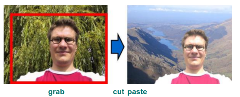
Graph segmentation: GrabCut

User helps the algorithm by selecting a box around the feature of interest

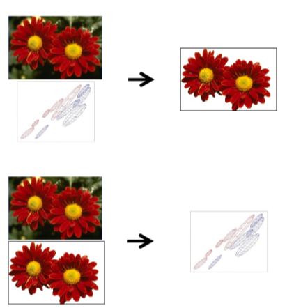
Graph segmentation: GrabCut process

1. Segmentation using graph cuts, requires having foreground model

2. Foreground-background modelling using unsupervised clustering, requires having segmentation

Improving efficiency of segmentation: Superpixels

Problem: Images contain many pixels (especially for graph-based)

• Group together similar-looking pixels for efficiency of futher processing

• Cheap, local over-segmentation

Important to ensure that superpixels…

• Do not cross boundaries

• Have similar size

• Have regular shape

• Algorithm has low complexity

Common definition of superpixel

Group of connected and perceptually homogeneous pixels which do not overlap any other superpixel

How to evaluate segmentation?

Use a ground truth made by a human

F = 2PR/(P+R)

Precision P: percentage of marked boundary points that are real ones

Recall R: Percentage of real boundary points that were marked