Applied statistics - Chapter 2: Measures of central tendencies & Describing and Organizing Data

Measure of central tendency

Summarizes data by describing the most typical (most representative) value in the distribution, center, or midpoint of a dataset

Mode

The most frequently occurring score in the distribution

Mode (con’t)

Is most often used to describe or interpret nominal-level data (is rarely useful for anything else)

e.g. Which news channel do most people prefer? 2, 2, 4, 4, 7, 7, 7, 7, 50, 50, 50. Mode = 7

Mode (III)

It likely reflects subgroups in the dataset

e.g. Yearly income of instructors in the psychology department: you would get a bimodal distribution, with graduate students making less than professors

Bimodal

When a distribution has two modes

Multimodal

When a distribution has more than two modes

Median

The midpoint of the distribution of scores, where ½ of the scores are below this point, and ½ of the scores are above it

Median (con’t)

Is primarily useful with ordinal-level data, but inappropriate for nominal-level data

Median (III)

Is more suitable for when extreme scores are present

Finding the median for an odd number of scores

1. Arrange scores from lowest to highest

2. Find the location (position) of the median in a data set: Add 1 to the number of scores (N) and multiply by .50 Location of Median = (N + 1) (.50)

3. Determine the actual value of the median: Start with the lowest score and count up the number of scores found in #2 above

Finding the median for an even number of scores

• The location of the median is halfway between the middle two scores.

• The actual value of the median is the sum of those two scores divided by 2.

Finding the median for an even number of scores (con’t)

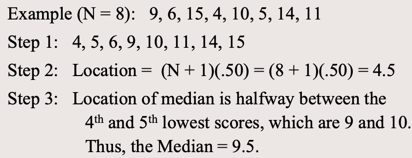
(N = 8): 9, 6, 15, 4, 10, 5, 14, 11 (arrange in order)

• Step 1: 4, 5, 6, 9, 10, 11, 14, 15

• Step 2: Location = (N + 1)(.50) = (8 + 1)(.50) = 4.5

• Step 3: Location of median is halfway between the 4 th and 5th lowest scores, which are 9 and 10. Thus, the Median = 9.5.

Mean

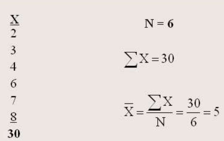
The ‘average’ of all the scores (Sum of scores divided by number of scores)

Mean (con’t)

Can only be used with interval or ratio level data

Mean example

How many scores fall below the mean

50% of scores fall below the mean

How many scores fall outside 2 standard deviations around the mean

5% of scores fall outside 2 standard deviations around the mean

68% Rule

The principle that in a normal distribution, $68\%$ of scores fall within one standard deviation above and below the mean.

95% Rule

The principle that in a normal distribution, $95\%$ of scores fall within two standard deviations above and below the mean.

What happens to the mean when the score value’s changed?

Changing the value of a score changes the mean

What happens to the mean when a new score’s introduced?

Introducing a new score or removing a score usually changes the mean (unless the score added or removed is exactly equal to the mean)

What happens to the mean when a constant is added or subtracted from?

Adding or subtracting a constant from each score changes the mean by the same constant

What happens to the mean when a constant is multiplied or divided from?

Multiplying or dividing each score by a constant multiplies or divides the mean by that constant.

Important properties of the mean

Summed deviations about the mean are always equal to zero.

• Deviation score: X - X

• If we were to sum (add) all of these deviation scores, the answer will ALWAYS, NO MATTER WHAT, be 0. [Sigma notation (X – X) = 0]

Important properties of the mean (con’t)

The sum of the squared deviations are least about the mean

The least squares concept

Using the mean to calculate the sum of the squared deviation scores (sum of Squares) will result in the smallest possible value for the sum of squares

Important properties of the mean (III)

The mean is very sensitive to extreme scores

The weighted mean

The overall mean from 2 or more different samples, and if one sample contributes more scores to the mean than the other

How to calculate the weighted mean

1. Multiply each group's mean by the number of people in that group.

2. Add up those products

3. Divide the sum of those products by the total number of people

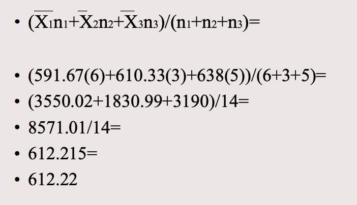
i.e. (X1n1+X2n2+X3n3)/(n1+n2+n3)

How to calculate the weighted mean example

Rats’ reaction time (light →bar press): three groups of rats, three different mean reaction times:

- N=6, X=591.67; N=3, X=610.33; N=5, X=638.00

• (591.67(6)+610.33(3)+638(5))/(6+3+5)=

• -3550.02+1830.99+3190)/14= • 8571.01/14=

• 612.215=

• 612.22

Univariate

When only 1 variable is involved

e.g. Frequency tables, pie/bar charts, histograms

Bivariate

When only 2 variables are involved

e.g. XY Scatter plots

Frequency distribution

An organized tabulation showing the number of individuals located in each category on the scale of measurement

e.g. A table or graph

Frequency distribution (con’t)

Always shows

• The categories that make up the scale

• The frequency, or number of individuals, in each category

F(X) in frequency distribution

Gives the number of times (or frequency) each score is seen in the data

X in frequency distribution

Lists all values of the score from highest to lowest

Calculations using frequency distribution tables

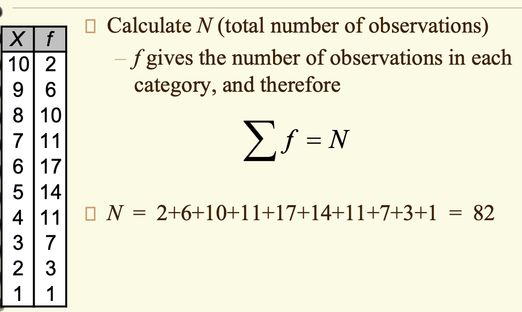
Calculate N (total number of observations)

• f gives the number of observations in each category, and therefore

Category

Represents a way of grouping together observations that are similar to one another

Category (con’t)

A list of the different possible values of the variable X

Class

A mutually exclusive category which represents elements or data points that share a common characteristic.

Frequency

The number of times a particular score, X, occurs in a data set

Frequency (con’t)

The frequency (or the number of values) in each class of the X variable. F(X)

Frequency distribution (III)

When the distribution shows the number of times each score occurs

i.e. Frequencies of the scores.

Grouped frequency distribution

Collapses the frequency distribution into mutually exclusive intervals or classes

Mutually exclusive

When each data point or X score can only be in one category

Relative Frequency (Proportion)

Converts frequency to relative frequency by dividing the frequency of a score or class by N (total number of scores)

Relative Frequency distribution

When scores are arranged in order of magnitude and the distribution shows the relative frequency for each score or point

i.e. The proportion of scores at each point

Percent (%)

Multiplying the relative frequency by 100

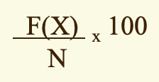
Percent Distribution

When scores are arranged in order of magnitude and the distribution shows the percent for each score or point

Proportion (p)

The fraction of all of the observations (N) that are associated with a specific score

Proportion (p) and percentage

A percentage is simply the proportion expressed as a %

Skew

Relative symmetry of a distribution of scores

Positive skew

A distribution in which scores are clustered at the lower end of the scale and tail off to the positive (higher) end of the scale

Negative skew

A distribution in which scores are clustered at the higher end of the scale and tail off to the negative (lower) end of the scale

Kurtosis

The degree to which scores are clustered about one common area of a distribution vs. distributed more so across or throughout the range of values

Kurtosis (con’t)

Curves are always symmetrical

Mesokurtic

A normal bell-shaped curve

Leptokurtic (Peaked distribution)

When scores are clustered/piled in one area

Platykurtic (Flattened distribution)

When scores are spread more evenly across the range of values

What are bar graphs best used for?

Nominal-level data (qualitative or categorical variables)

What are histographs best used for?

Ordinal-level, interval-level, or ratio-level data (quantitative variables)

Bar graphs

Is used for non-numerical values (scores)

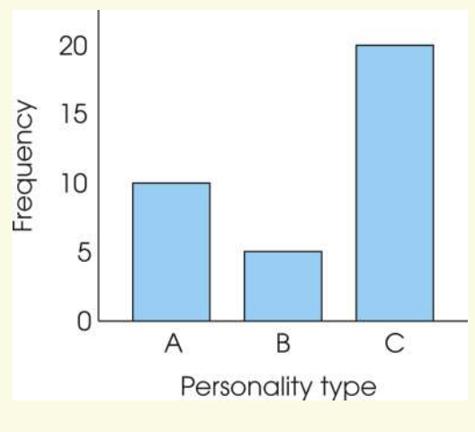
Bar graphs (con’t)

Spaces between adjacent bars indicates discrete categories without order (nominal) or of unmeasurable width (ordinal)

Bar graphs (III)

The Y-axis may represent score values, frequencies, percentages, etc.

Fundamental characteristics of a graph

• Two axes are drawn at a right angle.

• The horizontal axis is the X-axis (abscissa)

• The vertical axis is the Y-axis (ordinate)

• Both axes should have a value 0 where they meet

• Both axes should have relevant numerical values listed

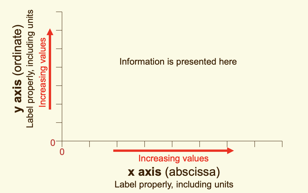
Fundamental characteristics of a graph (con’t)

• The independent variable is plotted along the X-axis

• The dependent variable is plotted on the Y-axis.

• The variables must be clearly labelled on both the X-axis and the Y-axis

• The graph should only contain all of the information needed to understand the data

Frequency distribution histogram

Is used to represent interval or ratio-level data

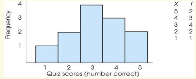
Frequency distribution histogram (con’t)

The X-axis represents a quantitative continuous variable

Frequency distribution histogram (III)

For continuous variables, rectangles represent class intervals

Class interval

A category of numbers with specified limits, and each number on the X-axis represents the MIDPOINT of a class interval.

Class interval (con’t)

Height corresponds to the frequency for that category

Pie charts

Are effective for displaying the relative frequencies of a small number of categories

Pie charts and catagories

The area of the slice is proportional to the percentage of responses in the category.

i.e. The relative frequency multiplied by 100.