5.6 - Production planning

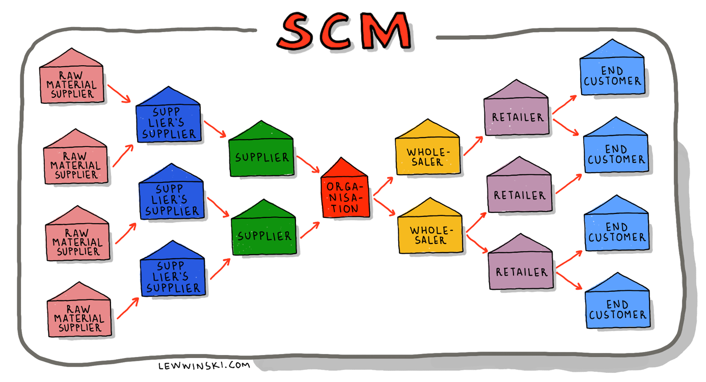
Supply chain

Supply chain is a series of processes involved in production and distribution of goods to the end customer or consumer.

• It can also be defined as a network of suppliers, producers and distributors.

• Regardless of the definition that you prefer, the key words here are process and network.

Supply chain management (SCM)

Supply chain management (SCM) refers to dealing with the flow of goods in the supply chain in the most efficient way. In other words, it is an area of management that is responsible for maximising the efficiency of the supply chain.

Local supply chain

Local supply chain is the one that operates on a smaller scale.

• Distances between suppliers, producers and distributors are relatively short.

• Local supply chains usually cover a region (province, city, town, county, or even neighbourhood).

• For example, production and distribution of fresh dairy products involves local supply chain: local farmers supply milk from local cows to local producers who then sell dairy products in local supermarkets.

• The main advantage of local supply chain is that local community benefits from it.

• The main drawback is limited choices — what’s available on a local scale is very limited compared to the global scale.

Global supply chain

Global supply chain is the one that operates on a larger scale.

• Distances between suppliers, producers and distributors are relatively long.

• Global supply chains are usually trans-national, which means that they involve several countries.

• For example, production and distribution of iPhones involves global supply chain: they are designed in the US, assembled in China and sold all over the world.

• The main advantage of global supply chain is that costs are minimised because organisations are able to find locations with the lowest labour or material costs in the world.

• The main drawback is high risk — organisations that operate globally have to rely on suppliers, manufacturers and distributors from different countries, with different legislation and culture and with different degree of political stability.

Stock (inventory)

Stock (inventory) refers to raw materials, components, work-in-progress (semi-finished goods) and finished goods that are held by organisations.

• For a fruit juice manufacturer, stock (inventory) might include oranges, apples, sugar, water, plastic bottles, etc.

Buffer stock

Buffer stock is inventory that is kept “just in case” (for demand fluctuations or for supply chain problems).

• For example, if juice manufacturer receives a sudden order for 1000 litres of orange juice and it had enough oranges in stock to produce that much of orange juice, those oranges would refer to a buffer stock.

Just-in-case

Just-in-case (JIC) is stock control system that holds buffer stocks.

• One of the main pros of this approach is the ability to use purchasing economies of scale by negotiating discounts with suppliers in exchange for purchasing higher quantities of goods or materials.

• However, since more things are held in stock, storage costs (insurance, security, utility bills, rent) are higher as well.

• JIC stock management allows to minimise the effect on demand fluctuations.

• If suddenly an organisation gets a special order to produce large quantities of output, there will be materials in stock to cater to this special order.

• But, JIC has negative effect on working capital because cash is tied up in stocks.

• Working capital is the difference between current assets and current liabilities.

• In other words, working capital is cash that is used to sustain daily operations.

• If cash is used to cover storage costs, then less cash is available for other things.

• And lastly, because of higher costs, break-even quantity would be higher for organisations that use JIC, compared to the ones that use JIT.

Just-in-time (JIT)

Just-in-time (JIT) is stock control system that aims at zero buffer stocks.

• Organisations that use JIT stock management have to rely on and develop close relationships with suppliers because JIT is impossible without swift deliveries from suppliers on short notice.

• Since there are minimal (or even zero) buffer stocks, storage costs (insurance, security, utility bills, rent) are low.

• However, if demand fluctuates suddenly, it might have a significant effect on the organisation.

• If, suddenly, an organisation gets a special order to produce large quantities of output, there might not be enough materials in stock to cater to this special order and suppliers might not deliver enough materials on short notice, so that special order might not be fulfilled.

• On the other hand, JIT has a positive effect on working capital because cash is freed up for day-to day operations, as opposed to being tied up in stocks.

• Additionally, because of lower costs, break-even quantity would be lower for organisations that use JIT, compared to the ones that use JIC.

Stock control

Stock control is the process of ensuring that appropriate amounts of stock are held. The two aims of stock control are:

• Meet customer demand without delay — make sure that customers always have an opportunity to purchase products at any time.

• Keep costs associated with stocks low — make sure that all the costs that are related to keeping stocks (insurance, utility bills, wages, etc) are minimised in order to maintain higher profitability.

Stockpiling

Stockpiling (keeping excessive levels of stock that are expensive to maintain)

Stockout

Stockout (the situation when stocks are insufficient to meet customers’ demand).

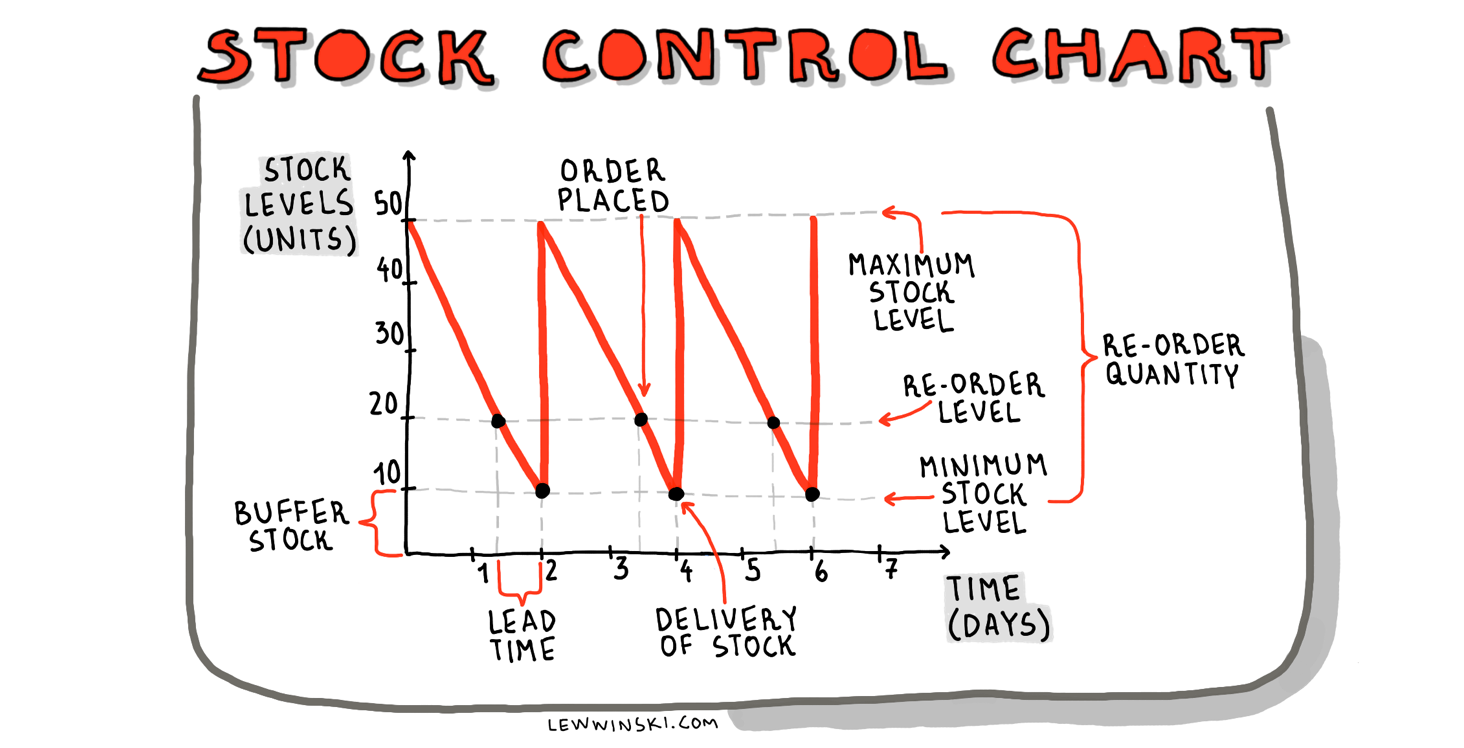
Stock control chart

Lead time is period between ordering new stock and receiving it. As you can see on the stock control chart, it is the interval between the actual delivery of stock and the time when the order was placed (i.e. when the stocks reached reorder level).

Buffer stock is minimum amount of stock. If stocks are at a level lower than the buffer stock, then production is compromised.

Reorder level is the level of stock at which the new order is placed. As you can see on the stock control chart, when stocks reach reorder level, order is placed and, ideally, supplies should be delivered before the stocks go lower than buffer stock level.

Reorder quantity is the amount of ordered stock. As you can see on the stock control chart, it is the difference between maximum stock level and buffer stocks.

Rates

• Capacity utilisation rate

• Defect rate

• Productivity rate

• Labour productivity rate

• Capital productivity rate

• Operating leverage

Capacity utilisation

Capacity utilisation is a measure of existing output relative to productive capacity.

Productive capacity is the maximum possible level of output. So, capacity utilisation rate expresses how much of productive capacity is used. The formula is:

Capacity utilisation rate = actual output ÷ productive capacity ⨉ 100

For example, if a school can accommodate 1000 students, but there are only 890, capacity utilisation rate is 89%.

Defect

Defect is a characteristic/fault/problem of a product that hinders its usability.

• For example, if you buy a new smartphone and its screen does not work, it is clearly a defect.

• However, in different industries there is different tolerance towards what is considered a defect, and what is just a feature.

• What exactly is considered to be a defect depends on quality standards. The formula for defect rate is:

Defect rate = number of defective units ÷ total output ⨉ 100

For example, if out of 50 chairs that XYZ manufactured, 2 have defects, then defect rate would be 4%.

Productivity

Productivity is a measure of efficiency of production.

• It is always relative to internal or external (competitors’) benchmarks, which means that simply knowing productivity rates of a certain organisation does not provide many insights unless it is compared to standards (benchmarks) and competitors. The formula of productivity rate is:

Productivity rate = total output ÷ total input

Keep in mind that this is a general rate that has to be contextualised, depending on the type of input. We’ve already learnt what inputs (or resources, or factors of production) : physical inputs (land), financial inputs (capital) and human inputs (labour). So, productivity rate can measure literally anything, as long as you are able to contextualise inputs and outputs.

• The next two rates (labour productivity and capital productivity) are two contextualised kinds of productivity rate, because they refer to specific types of inputs (human resources and financial resources accordingly).

Labour productivity

Labour productivity is a measure of worker’s efficiency.

• It can be applied to calculate a single worker’s productivity, or a group, or the entire workforce.

• Again, it all depends on the context and on organisational needs.

• Regardless, the formula is:

Labour productivity = total output ÷ hours worked

For example, if Ivan assembles 24 chairs in his 8-hour shift, then his productivity is 3 chairs per hour.

Capital productivity

Capital productivity is a measure of efficiency of organisation’s capital, especially working capital. Working capital is cash that is used to sustain daily operations of the business. Its formula is:

Working capital = current assets — current liabilities

Working capital productivity can be calculated using the formula below:

Working capital productivity = sales revenue ÷ working capital

If current assets in a balance sheet are worth $1000, current liabilities are $400 and sales revenue is $1200, then capital productivity is 2:1. It means that every dollar of working capital generates $2 revenue.

Operating leverage

Operating leverage is a measure of the effect of fixed costs on profit given different sales levels.

• This rate uses the same data as break-even analysis: fixed costs, variable costs, contribution.

• How to calculate contribution:

Unit contribution = P – AVC

Total contribution = (P – AVC) ⨉ Q

The formula of operating leverage is:

Operating leverage = total contribution ÷ profit

Change in profit (%) = change in sales (%) ⨉ operating leverage

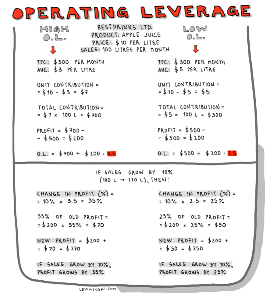
High operating leverage

High operating leverage is common for businesses with high levels of fixed costs.

• Usually, these are capital-intensive businesses that rely on machinery in production.

• On the one hand, high operating leverage means that more sales would lead to more profit.

• That is because fixed costs do not change with the increase in output, so the more output is sold, the higher the profits are.

• However, on the other hand, in addition to high levels of fixed costs, high operating leverage also implies higher risk if sales are low.

• That is because lower sales will not be able to cover fixed costs and thus they jeopardise profitability.

Low operating leverage

Low operating leverage is common for businesses with low level of fixed costs.

• Usually, these are labour-intensive businesses that rely on workers in production.

• On the one hand, low operating leverage implies low risk if sales are low.

• That is because most of the costs the organisation bears are variable.

• And if sales revenue is low, then variable costs are also low because they are proportional to the level of output (i.e. low output means low variable costs).

• However, on the other hand, more sales do not have much effect on profit.

• This is, again, because mosts of the costs are variable, so an increase in sales will have proportional increase in costs, thus not having as much of a positive effect on profitability, compared to high operating leverage.

Make-or-buy decision

Make-or-buy decision is a choice between purchasing from supplier and manufacturing on one’s own.

• For example, a pizza restaurant might face a make-or-buy decision if its managers are thinking whether to buy tomato sauce from a supplier or producing their own.

• Making this decision would involve consideration of some qualitative and quantitative factors.

• Qualitative factors might be supplier’s reputation and reliability, product quality, ethics.

• Quantitative factors might be break-even analysis, investment appraisal, budgets and costs: cost to buy (CTB) & cost to make (CTM).

Cost-to-buy (CTB)

Cost to buy (CTB) is the cost of purchasing from supplier. It is calculated by simply multiplying price per item bought from supplier by quantity:

CTB = P ⨉ Q

Cost to make (CTM)

Cost to make (CTM) is the cost of manufacturing on one’s own. It is calculated by adding all costs (fixed and variable) together.

CTM = (AVC ⨉ Q) + TFC

Pros and cons of CTM and CTB

• On the one hand, CTB and CTM are simple, quick, easy and helpful tools for making a make-or-buy decision.

• However, considering CTB and CTM only provides decision-makers with quantitative perspective, so qualitative factors should also be considered in make-or-buy decisions.

• In addition to evaluating CTB and CTM as decision-making tools, you might use them and qualitative factors to evaluate different make-or-buy decisions.