Law of Supply and Demand

Law of Supply

Price has direct relationship to Qs

Changes in Qs

• caused by a change in price

• shown as movement along curve

Price Variables (Supply)

• Profit Incentive

• Law of Increasing Opp. Cost

changes in supply

• caused by non-price variables

• shown as shift of the curve

Non-Price Variables

• SPENT

SPENT: S_____

Suppliers Input Price (inverse)

SPENT: P____

Price of related goods

SPENT: E____

Expectations

SPENT: N____

Number of sellers (direct)

SPENT: T____

• Taxes (inverse)

• Temperature

• Technology (increase)

• Tampering

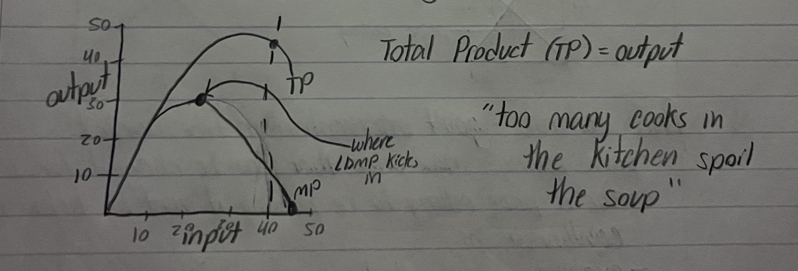
Law of Diminishing Returns or Diminishing Marginal Product

Add factors of production to fixed factors of production, total output increases initially but eventually the additional output diminishes to the point of negative returns

Elasticity of Supply

determined by time

• short-run vs long run

Short Term for Es

time frame in which some inputs are fixed

long-run for Es

time frame in which all inputs variable

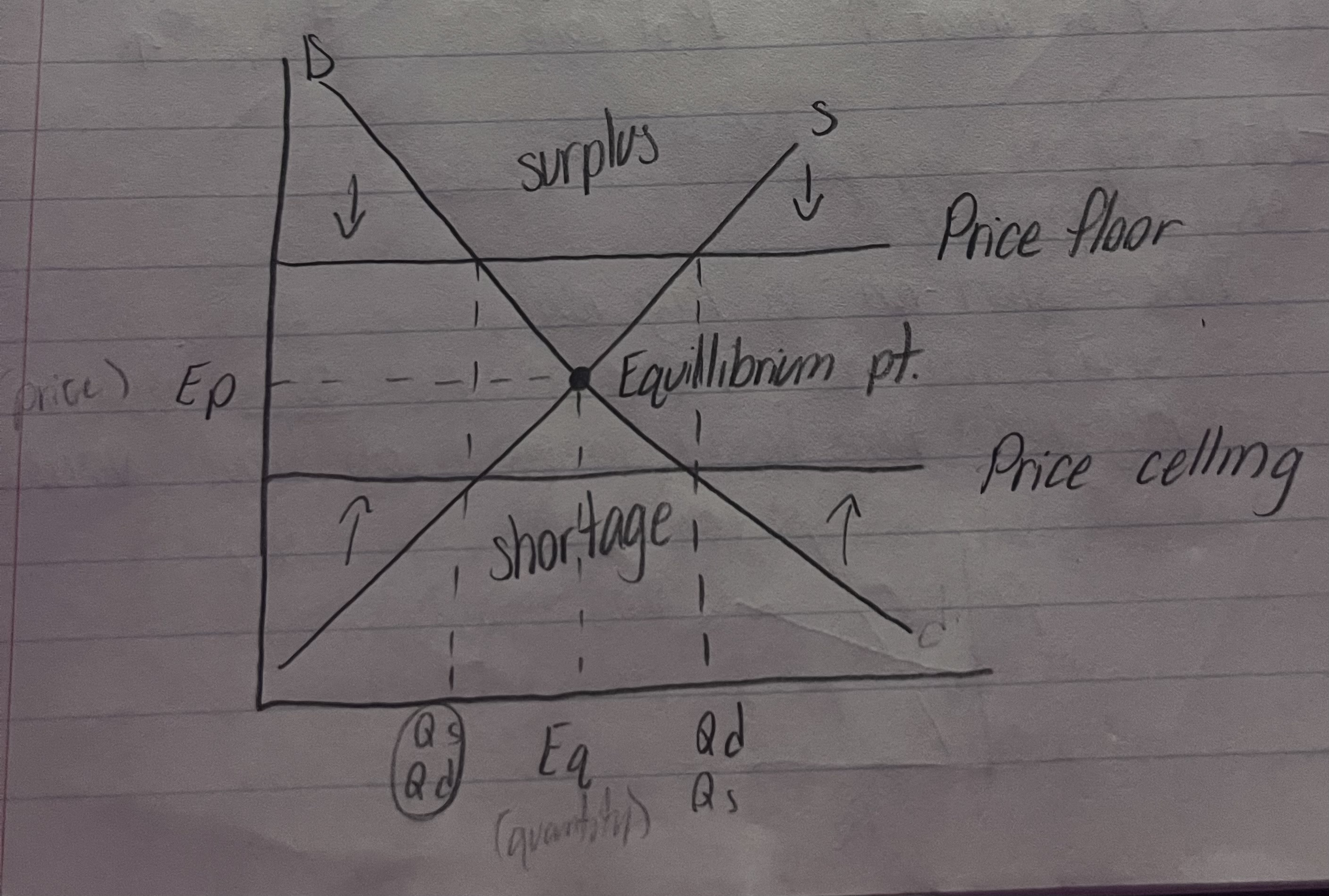
Market Equilibrium

where supply+demand intersect and sets market price + market output

Price Controls

gov’t intervention in free market

Price Celling

max price that can be charged for a g/s

• below equilibrium point

• rent control

• result - Qd > Qs = shortage

• consequence - slum lords

Price Flooring

minimum price that can be charged for a g/s

• above equilibrium point

• wage laws

• result - Qs > Qd = surplus (labor)

• consequence - increased unemployment

Market Equilibrium Graph

In Market Equilibrium: If demand increases

supply stays constant

price increases

quantity increases

In Market Equilibrium: If demand decreases

supply stays constant

price decreases

quantity decreases

In Market Equilibrium: If supply increases

demand stays constant

price decreases

quantity increases

In Market Equilibrium: If supply decreases

demand stays constant

price increases

quantity decreases

In Market Equilibrium: If both demand and supply increase

price stays constant

quantity increases

In Market Equilibrium: If both demand and supply decrease

price stays constant

quantity decreases

In Market Equilibrium: If demand increases and supply decreases

price increases

quantity stays constant

In Market Equilibrium: If demand decreases and supply increases

price decreases

quantity stays constant

Law of Demand

P-up Qd-down + P-down Qd-up; inverse relationship

Ceteris Paribus

basic assumption in law of supply+demand

means all other variables that can influence Demand remain constant

Changes in Qd

caused by change in price; shown as movement along the demand curve

3 Price Variables

Substitution Effect, Real Income Effect, and Law of Diminishing Marginal Utility (DMU)

Substitution Effect

When price of good X increases, then people buy more good Y; PRIMARY CAUSE

Real Income Effect

When price increases or decreases but income (Y) stays the same

Law of Diminishing Marginal Utility (DMU)

the more you consume of a g/s the less additional satisfaction received

The only way to consume more is to decrease price

Changes in Demand

caused by non-price variables and involve a shift in the demand curve

PYNTE - P____

Price of relates goods

PYNTE - Y___

Income

PYNTE - N____

Number of consumers (population)

PYNTE - T____

Taste and Preferences

PYNTE - E____

Expectations about a future change in price or event

Elasticity of Demand

responsiveness of changes in Qd to a change in price

Elasticity of Demand Coefficient (Ed)

Ed>1 = elastic

Ed<1 = inelastic

Ed=1 = unit elastic

*ignore negative value

4 determinants of Ed

1. Luxury (E) vs Necessity (In)

2. Can it be substituted? (yes=E, no=In)

3. % of income spent (large=E, small=In)

4. Time → increases elasticity

Midpoint Formula (Simplified) (Ed)

\frac{Q2-Q1}{Q2+Q1}\cdot\frac{P2+P1}{P2-P1}

Total Revenue Test of Elasticity

Elastic = P-up TR-down + P-down TR-up

Inelastic = P-up TR-up + P-down TR-down

Cross Elasticity

measures the impact of change in price of goods x, on the change in demand of goods y

Cross Elasticity Formula (Exy)

% change D y / % change P x

negative value = complementary

positive value = substitutes

Income Elasticity

measures the change in D in response to a change in income

Income Elasticity Formula (Ey)

% change in D / % change in Y

negative value = inferior good

positive value = normal good

perfectly inelastic

perfectly elastic