!! Bulk, Single Cell, and Spatial RNA-Seq

Why study RNA?

• RNA is dynamic, capturing more information than static DNA.

• RNA is the first quantitative link between DNA sequence and phenotype.

• RNA capture regulatory complexity beyond gene sequence.

  • The transcriptome encodes layers of control not visible in DNA through alternative splicing and noncoding RNA regulation.

Gene expression

• A gene is a short DNA section containing instructions for making proteins.

  • Exons, introns.

  • Alternative splicing.

    • Different combinations of exons.

    • Multiple transcripts.

• Gene expression level is the number of gene transcripts produced in an organism or cell.

• It’s the process of using DNA information to create RNA and proteins.

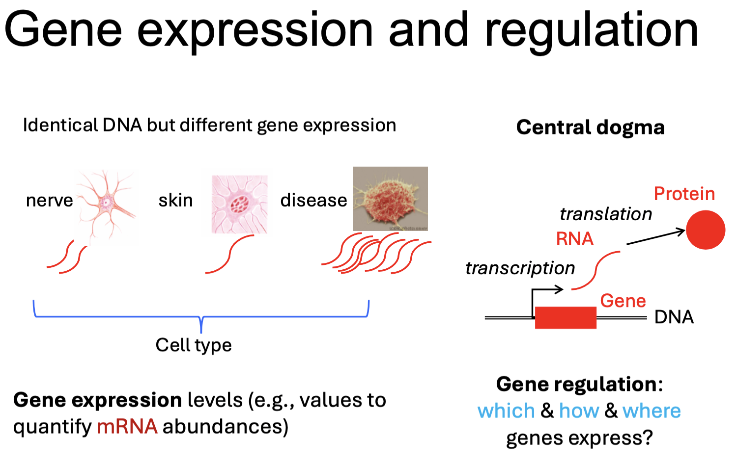
Detecting gene expression

• RNA-Seq and DNA microarray can be used to profile gene expression.

• cDNA (complementary DNA) is used in gene expression studies to detect and quantify gene expression products.

  • RNA is not stable and can be easily degraded.

• cDNA libraries are gene libraries containing only genes expressed in a cell or tissue.

RNA-Seq steps

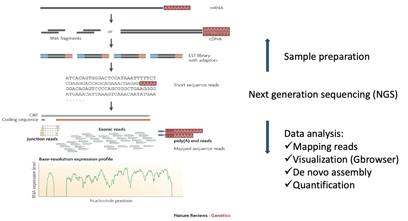
1. Sample preparation: Prepares the mRNA for sequencing.

   • Starting material: Total RNA is isolated, explicitly focusing on the mRNA.

   • Fragmentation/cDNA synthesis: The mRNA can either be fragmented directly into RNA fragments or be converted into more stable cDNA using reverse transcriptase.

   • Adapters: Sequencing adapters are ligated (attached) to the ends of fragments, creating a sequencing library.

2. Next Generation Sequencing: The prepared library is sequenced to produce raw data.

   • Sequencing: The fragments are sequenced to generate millions of short sequence reads.

3. Data analysis: The raw sequencing reads are processed to quantify gene expression.

   • Mapping reads: The short reads are aligned against a known reference genome or transcriptome.

     • Exonic reads map entirely within an exon.

     • Junction reads span a splice junction (connecting two exons).

     • Poly(A) end reads map to the end of the transcript, confirming the 3’ end.

   • Visualization (genome browser).

   • De novo assembly: If a reference genome is unavailable, reads can be assembled to build transcripts.

   • Quantification: he number of reads mapping to a gene or transcript is counted to determine its expression level. The final result is a Base-resolution expression profile, a graph showing the abundance of RNA (read coverage) across the transcript length.

RNA-Seq analysis steps

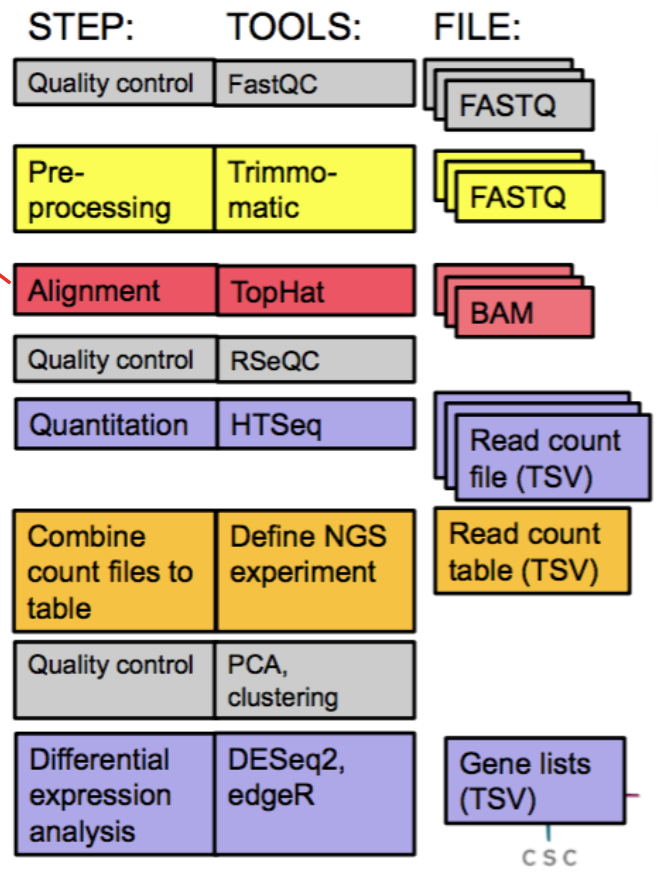
• Quality control sequence output = FASTQ files.

• Pre-processing notes: If the reads contain low-quality bases or adapter sequences, you might want to trim or filter them.

• Alignment notes: map reads to reference genome/transcriptome; output = BAM files.

• Quantitation notes: abundance quantification; gene, exon, or transcript levels.

RNA read alignment

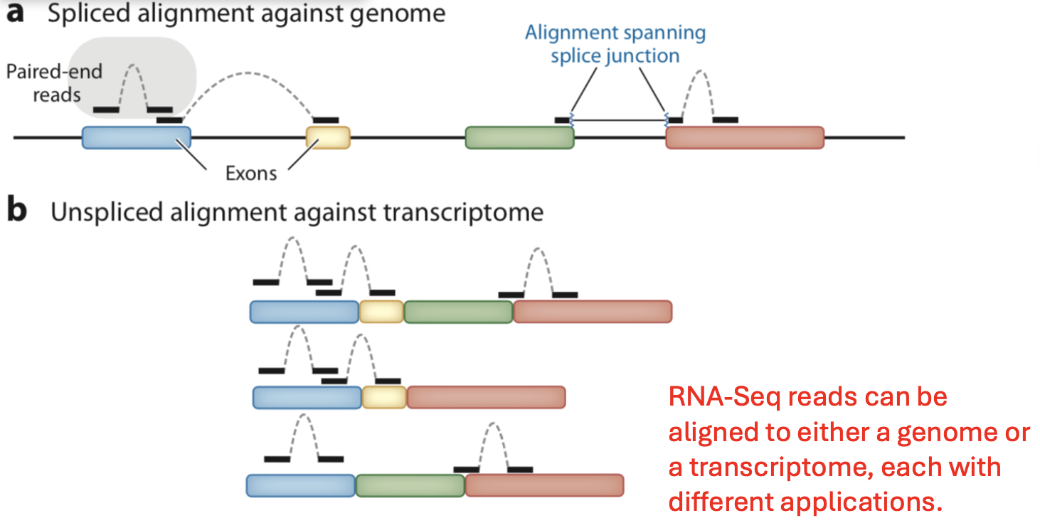
• Find the position of a sequencing read on the reference genome.

  • Reads can be unaligned or aligned to more than one location.

  • A paired-end read will only be counted as one read if both ends align to the genome.

• Given a list of transcripts, each read can be mapped to one of the four classes: exonic, partially overlaps an exon, intronic, or between genes.

  • Why intronic: They are mostly unspliced pre-mRNA or functional non-coding RNAs transcribed from those genomic regions.

Abundance quantification

• Raw counts can be biased:

  • Sequencing depth: Different total numbers of reads between samples.

    • Correction: Normalizing by total library size.

  • Gene length: Longer genes have more space for reads to map, leading to higher raw counts even if the gene's concentration is the same as a shorter gene.

    • Correction: Normalizing by transcript/gene length.

  • RNA composition: A few highly expressed genes can take up a significant fraction of the total reads, making other genes appear to have lower expression than they really do. This affects the comparison between samples.

    • Correction: Using specialized between-sample normalization methods.

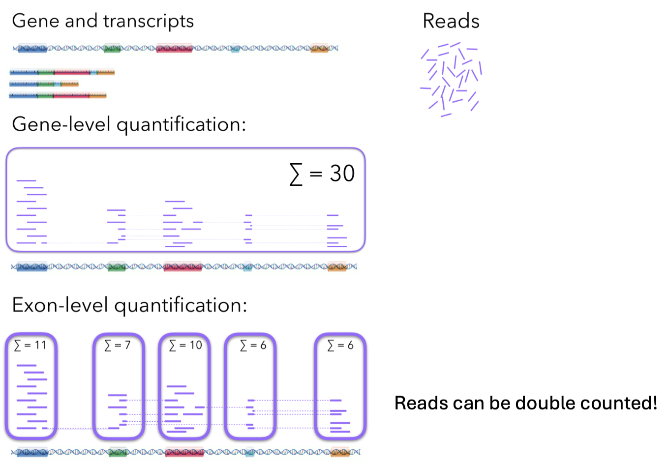
RNA-seq normalization methods

• Within sample:

  • Required to compare the expression of genes within an individual sample.

  • It can adjust data for two primary technical variables: transcript length and sequencing depth.

• Counts per million (CPM).

• FPKM (fragments per kilobase of transcript per million fragments mapped).

• Transcripts per million (TPM).

Counts per million (CPM)

• The number of raw counts mapped to a transcript, scaled by the total number of sequencing reads in your sample, multiplied by a million.

• It normalizes RNA-seq data for sequencing depth but not gene length.

  • Not yet ready for comparison of gene expression.

FPKM (fragments per kilobase of transcript per million fragments mapped) & RPKM (reads per kilobase of transcript per million reads mapped)

• FPKM = paired-end data.

• RPKM = single-end data.

• Correct for both library size and gene length.

• Good for comparison of gene expression within a single sample, but not for across-sample comparison.

Transcripts per million (TPM)

• Represent the relative number of transcripts you would detect for a gene if you had sequenced one million full-length transcripts.

• Correct for both sequencing depth and transcript length.

• Suitable for within-sample comparison of gene expression, but not for across-sample comparison.

RPKM summary

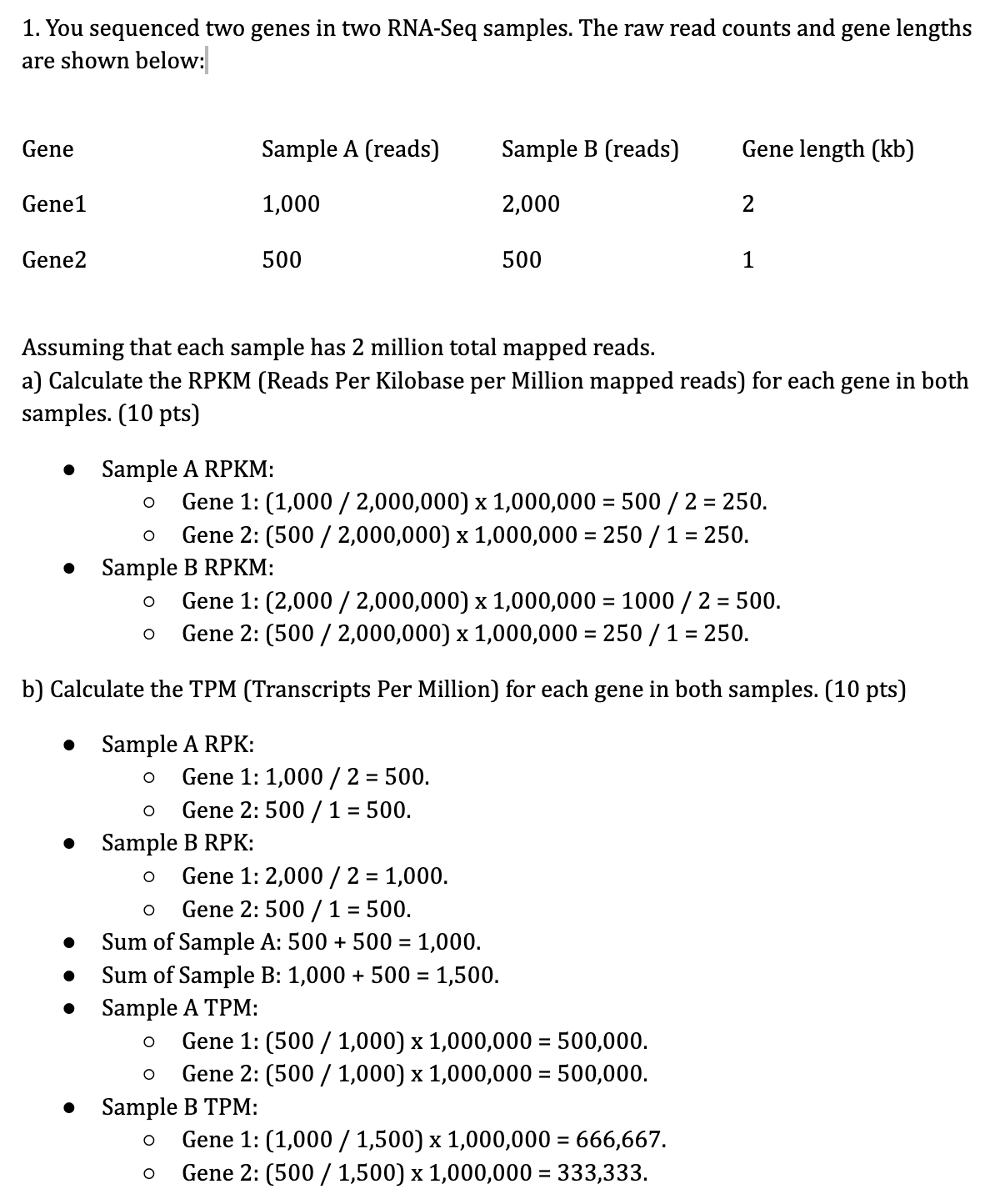
• Step 1 = normalize for sequencing depth: RMP = (raw counts for gene / (total mapped reads / 10)) x 1,000,000.

  • Divide the total mapped reads by 10 to simplify the number.

• Step 2 = normalize for gene length: RPKM = RPM / gene length in kilobases.

• Example:

  • Gene length = 2 kb.

  • Gene raw counts = 10.

  • Total mapped reads = 35.

  • Step 1: (10 / (35/10)) x 1,000,000 = 2.86.

  • Step 2: 2.86 / 2 = 1.43.

TPM vs. RPKM

• RPKM:

  • Reads mapped / (gene length * total mapped reads in millions).

  • Normalizes for depth first, then length.

  • The total RPKM/FPKM of all genes in a sample does NOT sum to the same value across different samples.

  • Only for comparing the expression between different genes within a single sample.

• TPM:

  • ((Reads mapped / gene length in kb) / (sum of all genes) (reads mapped / gene length in kb)) * 10⁶.

  • Normalizes for length first, then scales the length-normalized values (the RPK) by the total sum of all RPKs in the sample.

  • The sum of all TPM values in a sample is always 106 (one million), making samples directly comparable.

  • Recommended for comparing the expression of a single gene across different samples (replicates).

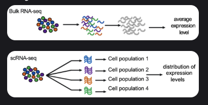
Evolution of gene expression measurements

• Bulk RNA-seq: Measures average gene expression across many cells.

  • Cost-effective and straightforward, but masks cell-to-cell differences.

• Single-cell RNA-seq: Profiles individual cells to reveal cellular heterogeneity, rare cell types, and dynamic states.

• Spatial RNA-seq: Captures where genes are expressed within tissue, preserving spatial context and cell-cell interactions.

Why study single cells?

• When compared to bulk RNA-seq, single-cell studies:

  • Reveals cell-to-cell differences and provides an unbiased view of cellular complexity within a tissue.

  • Allows for the discovery and precise identification of rare cell types and dynamic cellular states (e.g., transitional stages).

  • Provides the highest resolution view of the intermediate step between genotype and phenotype (where cells are the functional constituents).

Bulk vs. scRNA-seq

• Bulk RNA-seq:

  • Quantifying expression signatures from ensembles.

  • Insufficient for studying a heterogeneous system.

• scRNA-seq:

  • Inference of gene regulatory networks across the cells.

  • Heterogeneity of cell responses.

  • Cell type identification.

scRNA-seq analysis cell- and gene-level analysis

• Cell-level:

  • Marker gene identification.

  • Cluster analysis.

  • Trajectory analysis.

• Gene-level analysis:

  • Single-cell differential expression analysis.

  • Gene set analysis.

  • Gene regulatory networks.

scRNA-seq process

1. Sample preparation.

2. Single-cell RNA sequencing.

3. Data processing.

4. Data analysis.

scRNA-seq sample preparation

• Cells are physically separated into a single-cell solution from which specific cell types can be enriched or excluded.

  • Each cell is captured by one droplet.

  • Each droplet contains a unique barcode and the necessary reagents for reverse transcription.

  • Each individual RNA molecule captured within that droplet is tagged with its own unique molecular identifier (UMI).

    • The UMI distinguishes unique RNA molecules from duplicates that arise during PCR amplification.

scRNA-seq single-cell RNA sequencing

• Extremely small amount of RNAs within a cell → hard to detect.

• PCR amplification → start sequencing.

scRNA-seq data processing

• UMI.

• Gene counts.

• Drop-outs in single cell.

• Imputation method: MAGIC.

Unique molecular identified (UMI)

• UMIs are short (4-10 bp) random barcodes added to transcripts during reverse-transcription.

• UMIs enable sequencing reads to be assigned to individual transcript molecules and thus the removal of amplification noise and biases from scRNA-Seq data.

• They reduce the amplification noise by allowing (almost) complete duplication of fragments.

• Counting the number of distinct UMI sequences is easier.

• This information does not get lost during the amplification process.

Gene counts

• In each gene, within each cell, the total number of unique UMI is counted and reported as the number of transcripts of that gene for a given cell.

Drop-outs in single cell

• A gene can be observed at a moderate or high expression level in one cell but not detected in another.

• Why do dropouts occur in a single cell:

  • Technical artifacts.

  • Cell type differences.

  • Statistical sampling.

  • Biological factors.

• Zero inflation: unusually high number of zeros (undetected gene expression values).

What should we do about dropouts?

• Ignore zero inflation:

  • Let downstream statistical methods do the heavy lifting.

• Aggregate information across similar cells.

  • Clustering or pseudobulk approaches.

  • Smooth out noise and highlight consistent expression patterns.

• Impute scRNA-seq gene count matrix before analysis.

  • Estimate missing gene expression values and reduce sparsity caused by dropouts.

Why do we need imputation methods?

• Downstream analyses rely on the accuracy of gene expression measurements.

• Imputation methods:

  • MAGIC.

  • Droplet.

  • DrImpute.

  • scDoc.

MAGIC (Markov affinity-based graph imputation of cells)

• Denoise high-dimensional scRNA-seq data.

• Impute missing expression values by sharing information across similar cells.

• Transform the similary of matrix A into Markov transition matrix M.

• Raise the Markov matrix to the power of t: M^t, which determines the weight of cells.

scRNA-seq data analysis

• Dimensionality reduction.

• Clustering and marker identification.

• Trajectory analysis.

Gene expression analysis: clustering

• Organize objects into groups based on similarity.

• A cluster is a collection of objects which are similar to objects in the same cluster, but are dissimilar to objects in other clusters.

Hierarchial clustering

• Divisive:

  • Starts with all data points in one cluster.

  • Choose split so that data points in the two clusters are most similar (maximize “distance” between clusters).

  • Continue until all data points are in single gene clusters.

• Agglomerative: union between the two nearest clusters.

  • Start with each data point in its own cluster.

  • Joins the two most similar clusters.

  • Continues until all data points are in one cluster.

How to find the two most similar clusters

• Single linkage: shortest distance.

• Complete linkage: longest distance.

• Average linkage: average distance.

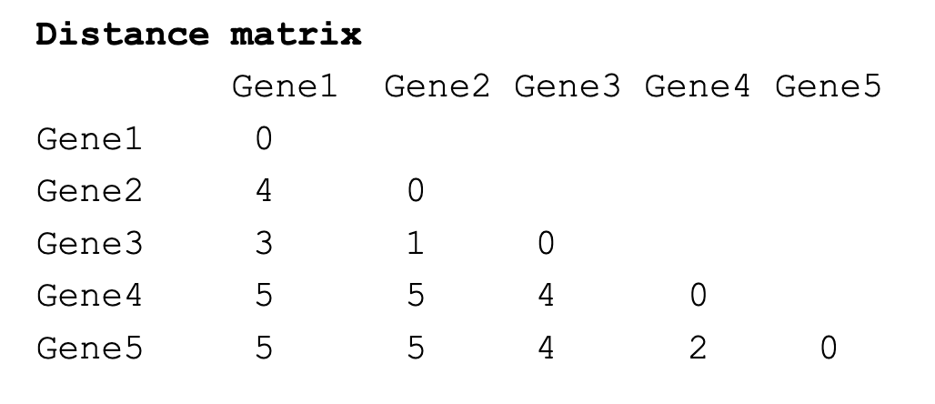
!! Single-linkage example

ask gemini

!! Biclustering

• Clustering becomes too restrictive on large datasets:

  • Seeks a global partition of genes based on their expression similarity across ALL conditions.

• Relevant knowledge can be revealed by identifying genes with a typical pattern across a subset of the conditions: e.g., genes co-expressed under some conditions.

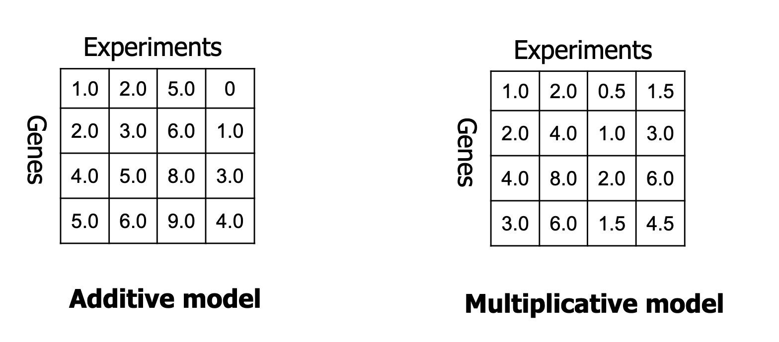
Bi-clustering patterns

• Constant values: might be an over/under-expression of a group of genes in a subset of experiments.

• Constant rows: a gene signature of a subset of experiments.

• Constant columns: a set of co-expressed genes in a subset of experiments.

• Coherent values: a common trend in a group of genes in a subset of experiments.

  • The picture holds examples.

!! A good bi-cluster

!! δ (Delta) bi-cluster

• Find bi-clusters with mean squared residue < δ.

• Repetitive procedure:

  • Remove the row/col that reduces H the most.

  • Add rows/cols that do not increase H.

  • Stop when H < δ.

• Mask bi-cluster with random values.

• Repeat to find more bi-clusters.

WHAT IS δ AND WHAT IS H????

!! Differential gene expression

What to compare - differential gene expression

• TPM: correct for sequencing depth and gene length.

  • Tool: edge, suitable for small sample sizes.

• TMM: correct for differences in transcript pool composition; extreme outliers.

• logCPM: stabilize variance; remove dependence of variance on the mean.

  • Tool: Limma, suitable for moderate to large sample sizes.

• All aim to provide better comparison across samples.

• Other tool: DESeq2.

  • Negative binomial model with geometric size-factor normalization; shrinkage of dispersion & fold-change.

  • Broadly used.

Normalization in differential gene expression analysis

• EdgeR, DESeq2, and some others want to keep the integer read counts in the differential gene expression testing because they:

  • Use a discrete statistical power.

  • Want to retain statistical power.

  • But they are simplified as part of the differential gene expression analysis.

• Limma is fine with continuous values like FPKM.

!! Parametric vs. non-parametric

• Parametric methods often work better.

• For experiments with fewer than 12 samples per group: use edgeR.

  • UseDESeq2 otherwise.

WHAT IS PARAMETRIC VS. NON-PARAMETRIC???

!! Be careful with DE analysis

• Too many false positives.

• Take-away message:

  • Wilcoxon rank-sum test is recommended.

    • what the hell is this