AP micro!!!!!!!!!!!

consumer theory

the study of how people decide to spend their money based on their individual preferences and budget constraints

positive vs normative

positive - fact based

normative - emotional theoretical

individual property rights

individual property rights cause people to use their stuff for what they decide is best, so it creates products considered valuable for the market

income / substitution effects

income effect: people buy good A because its price went down and they have more money left over after buying it

substitution effect: people buy more A because its price went down and is cheaper relative to its substitutes

why demand downslopingg

income + substitution effects along with law of diminishing MU

changes in price

changes in price shift ALONG demand curve

for opportunity cost comparisons

compare how much you give up. so for 1 apple you give up 2 oranges, so apple = 2 o / 1 a

law of demand + supply

d has inverse relationship w price, supply has direct

purchase more when price decrease bc

purchasing power increase

rationing function of prices

When the supply of a good is limited, its price increases, which can help to reduce demand and allocate the available quantity to those who are willing and able to pay the higher price.

price ceilings and floors (shortage, surplus, DWL, CS, PS)

• for shortage / surplus, look at supplier since shortage or surplus is based on what they produce 

  • price floor = surplus 

  • price ceiling = shortage 

• price ceiling: price is too low, so producers literally cannot produce more and make a profit. they will only produce at Q1 even tho people want more, so shortage 

• price floor: price is too high, so in order to make a profit producers will want to keep producing more and selling more, even if they can’t. so they’re producing at more than equilibrium and it’s not being bought, aka a surplus 

• DWL is the same for ceilings and floors, it’s the change in Q times gap between S and D times 1/2. 

• Ceilings have more consumer surplus bc of a lower price 

• Floors have more producer surplus bc of a higher price 

• Price floor w gov support means that gov buys excess surplus, so everything before equilibrium and under price is PS. everything beyond equilibrium and above demand curve is DWL.

how curves shift with externalities

• supply is kinda backward but for production externalities, a positive one means society faces a lesser cost and WANTS MORE (MSC shifts forward). a negative one means society faces a greater cost and WANTS LESS (MSC shifts back) 

• demand is straightforward for consumption externalities, a positive one means society has greater benefit and WANTS MORE (MSB shifts out). a negative one means society has a lesser benefit and WANTS LESS (MSB shifts in). 

• DWL is just difference in Q times difference in MSC/MPC or MSB/MPB times 1/2 

• quantity of society = quantity of producer means no DWL

Marginal external benefit

vertical distance between 2 supply curves

classifying goods

• two categories are whether you can exclude and whether people consume at same time 

• pure, private goods 

  • excludable and one person  

• toll goods (quasi-public goods) 

  • excludable but many people   

• common resources 

  • non excludable but one person  

• pure public good 

  • non excludable and many people 

cs / ps and how that is maximized / what it does

• maximized at allocative efficiency (P = MC and MB = MC)

• CS: summation of differences between price and how much someone is willing to pay 

• PS: summation of differences between price and for how much a firm is willing to sell 

• total surplus is a measure of wellbeing of a market

government failure

• can be when government intervenes to correct market failure but ends up making it worse 

• everything else like corruption, inefficiency, principal agent problem 

  • An agent may act in a way that is contrary to the best interests of the principal

TR Test

• Inelastic demand : TR correlates directly with price

• Elastic demand = TR correlates inversely with price

elasticity of supply and demand - measures if a change in price affects change in quantity more or less than the change in price

• formula: abs value of percent change in q over percent change in p

  • quesadilla goes in through top and comes out through bottom as poo 

  • greater than 1 is elastic, between 0 and 1 is inelastic 

  • 0 is perfectly inelastic, 1 is unit elastic, infinity is perfectly elastic

cross price elasticity - measures if X and Y are inverse or direct 

• percent change in Qx over percent change in Py 

• greater than 0 is substitutes, less than 0 is complements, equals 0 is independent

income elasticity of demand - measures if X and price are inverse or direct

• percent change in Qx over percent change in real income 

• greater than 0 is normal, less than 0 is inferior 

elasticity of resource demand

percent change in Q res over percent change in P res

if a firm experiences diminishing returns

if a firm experiences diminishing returns, MP decreases and MC will increase because it’s a reflection of MP. MP does NOT increase at a diminishing rate because its marginal, its already a rate

relationship between rate of decline of MU and elasticity

if MU decreases slowly, good is more elastic

profits (econ, acc, normal)

• econ prof = acc profit - implicit costs

• also econ prof = total revenue - explicit costs - implicit costs 

• pos acc profit means you’re making more revenue than explicit costs (not necessarily exactly more by amount of implicit) 

• pos normal profit means zero econ profits, so you’re making same revenue as explicit and implicit costs (so more than explicit by exactly as much as implicit) 

• pos econ profits means you’re making more revenue than explicit and implicit costs 

• anything that is forgone is implicit so even like taking out money that was used for forgone business, that’s all implicit

when are costs variable

all resources and costs are variable in the long run

cover what before what

cover variable costs before fixed cost bc we shutdown if we can’t cover var costs

LRATC intervals

• econ of scale: interval of LRATC where incr input by percent, outputs incr by more than percent 

• constant returns to scale: interval of LRATC where incr input by percent, outputs incr by percent 

• diseconomies of scale: interval of LRATC where incr input by percent, outputs incr by less than percent

• 

characteristics of different types of firms

• PC: large number of firms, standardized product, no non-price competition, no barriers to entry, no price setting control, constant cost industry 

• Monopoly: 1 firm, unique product, barriers to entry, public relations, price maker 

• Monopolistic competition: large number of firms, different products, easy entry, ads, some price control 

• Oligopoly: few firms, product can be standardized or differentiated, significant barriers to entry, price control w interdependence

• 

other things to note relating to these firms (alloc + prod eff, econ profit, which curves)

• for all, always check if you’re under AVC bc then you shut down 

• aloc eff (P = MC): PC, monopoly w price discrimination 

• prod eff (P = MIN ATC): PC

• PC and Monopolistic competition make ZERO ECON PROF 

• Monopoly (with amd without price discrimination) and oligopoly make POS ECON PROF 

• all of these graphs DO have ATC, and MC goes through min ATC for all of them

long run supply curve

increasing cost industry: upsloping because as firms enter, D increases, so resource costs go up, which means AVC goes up. so instead of price going back down to og equilibrium, it goes to equilibrium at new AVC, which is at a slightly higher price.

what happens when firms enter mkt

supply changes bc # of firms change which changes price back to 0 econ prof

PC

• 

• very few markets are actually PC 

• demand most elastic

• prof eff 

• alloc eff 

• horizontal D, no supply

monopoly

• 

• PS is from price to MC curve 

• CS is from price to D curve 

• DWL is from difference in Q from D to MR 

• not alloc eff or prod eff 

• demand middle elastic 

• left side of D curve is elastic range, right is inelastic. monopolies want to produce were D is elastic (MR positive) 

• because MR is downsloping, an increase in MC means an increase in price and a decrease in quantity 

• TR maxxed when MR = 0

taxing/subsidizing a monopoly

• per unit tax: MC shifts up , affects q 

• per unit subsidy: MC shifts down , affects q 

• lump sum tax: ATC shifts up bc affects fixed costs only , doesn’t affect q 

• lump sum subsidy: ATC shifts down bc affects fixed costs only , doesn’t affect q

natural monopoly

• 

• unregulated, it produces where MR = MC and goes up to D like normal 

• since ATC is always above MC, if we forced the output where P = MC, they would be making a negative econ profit 

• what you do is give them fair return pricing so they earn 0 econ profit at D = ATC 

• MC is either severely downsloping or horizontal, and below ATC 

• because a natural monopoly has a constantly decreasing ATC, it can supply its product at a lower cost than PC

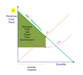
monopoly w price discrimination

• 

• alloc eff but not prod eff

• profit and output increase 

• produce where d = mc, all cons pay their highest price willing to pay (no PL) 

• econ profit is like the trapezoid between MC - ATC at Q, Price, and upper corner of graph

  • 1: charge customers max price willing to pay 

  • 2: charge one price at first, and less w each unit purchased 

  • 3: charge dif customers dif prices

alloc eff, socially optimal, prod eff, fair return

• allocatively efficient: p = mc 

• socially optimal: p = mc 

  • subsidies 

  • reduce but not eliminate DWL 

• productively efficient: p = min atc 

• fair return : p = atc 

  • no subsidies 

  • if you want a monopoly to make 0 econ profit 

  • reduce but not eliminate DWL

monopolistic competition

• 

• D tangent to ATC 

• no prod eff (P = atc but not min atc) 

• no alloc eff 

• demand least elastic 

• MC downward sloping demand curve is because differently valued products have diff prices 

• how is LR equilibrium achieved for Monop Comp

  • if the firm is making a profit, other firms will enter

  • the demand of each firm shifts down because now there is other firms to choose from and there are now more substitutes

  • demand keeps shifting down until it is tangent to ATC at minimum ATC point

4 firm concentration ratio 

• formula: add the market shares of the four largest firms

• 0 is PC 

• between 0 and 40 is MC

• greater than 40 is oligopoly

herfindahl index

• formula: square the market share of each firm competing in the market and then sum the resulting numbers

• 0 is PC 

• 10,000 is monopoly 

• the greater the index, the more oligopolistic it is

oligopoly

• 

• very sticky price + output 

• competing firms will match price cuts but not price increases 

• D is elastic above p1 because consumers will heavily take into account price and will move around, since there will be lower prices 

• D is inelastic below p1 because all companies have the same price and it doesn’t matter to consumers 

• dominant strategy: a firm will choose the same thing regardless of what the other chooses 

• nash equilibrium: state such that if either firm switches, they will lose 

• usually, if both don’t have a dominant strategy, there are 2 nash equilibria, but if they both do, there’s usually 1 nash equilibrium 

• no prod eff 

• no alloc eff

excess capacity in monop comp

• the gap between min-ATC output and profit maxxing output 

• the amount of underusedness of equipment bc its not producing at min ATC q 

• product differentiation incr demand

• 

business flow model

• 

• factor market is the exchange of resources for income 

• product market is the exchange of money for G/S

derived demand

• the demand for resources is determined (derived) by the products they help to produce.

mrp theory

• mrp: a resource is only as valuable as the amount of money it adds to revenue 

• mrp = change in TR over change in q of resource 

• mpp = change in q of product over change in q of resource 

• p times mpp equals mrp 

• mrp is firm’s resource demand curve 

• mrp is steeper sloping in an imperfectly competitive market

MP vs MC

• MP - how much product from adding one more resource

• MC - how much cost from producing one more output

• MC and AVC deal with output, MP and AP deal with resources

MRC and MFC are

the same thing

Resource market is what

Resource market is PC, produce where MRC = MRP

optimal is

optimal is when MP of labor over P of labor = MP of capital over P of capital

profit maxxing is when both of those equal 1

labor markets

• like a regular PC except S is horizontal instead of D. hire until wage (MRC) = MRP

• downward sloping d, horizontal supply (opposite from PC) 

• 

industrial union

just a higher wage (horizontal supply curve) until you hit real supply curve, then go up with it

monopsony

• single buyer of a resource 

• MRC above S curve, find where MRC = MRP and go down to supply 

• least cost: MP L over MRC L = MP C over MRC C 

• profit max: when both of those equal 1 

• hire less + pay less 

• MRC is greater than supply curve bc you have to pay more to each successive worker 

bilateral monopoly

• 1 union + 1 monopsonist 

• has the supply curve of a union where it’s weirdly high until it means S curve and goes up with it 

• wage will be anywhere between what the union wants, its artificial Wu, and what the monopsonist wants, which is equilibrium of monopsonist

• 

effects

• union - hire less pay more 

• monopsony - hire less pay less 

• bilateral monopoly - hire more pay more

Rent

• price paid for the use of land or other natural resources that are fixed in supply 

• rent is a surplus payment (econ rent), which is the payment above what is necessary to make a resource available for use 

• not a cost to society, but to individual producers

time value of money

• FV = P(1+i)^t which is equation we know 

• value of money decreases as time goes on 

• pure rate of interest

• 20 yr treasury bond 

Usury laws

regulations that limit the maximum interest rate that can be charged on loans or other financial transactions.

econ profit

portion of acc profit that is above average rate of return in the industry

LF Graph vertical axis

• real interest rate ( r )

different kinds of taxes

• progressive: average tax rate increases as income increases 

• proportional tax: avg tax rate is constant as income incr 

• regressive: avg tax rate decreases 

• 

tax graph

• govt revenue from a tax is the amount of tax (difference in curves) times Q produced. DWL is the space between the two Q’s that is in between D and og S. tax borne by cons is above P, tax borne by prod is below P. uncollected revenue loss is the rectangle between two Qs that goes up to Pe. inelastic demand/supply has less URL. 

• tax always effects supply 

• cons bear more of inelastic demand and elastic supply 

• prod bear more of elastic demand and inelastic supply (Draw it out)

• 

taxes

• marginal tax rate: the tax rate for each bracket. delta t over delta i 

• average tax rate: total tax paid divided by total taxable income 

• tax liability: amount taxed 

quota

expenditures federal state local

• federal: pensions, medical care 

• state: education, welfare 

• local: education, public safety, welfare 

revenue federal state local

• federal: personal income tax, payroll tax 

• state: sales/excise taxes, personal income tax 

• local: property taxes, sales/excise taxes

merging

• vertical: companies at different stages in the production process  

• horizontal: companies within the same industry

• conglomerate: companies in different industries or physical locations

gini coefficient

• area between line of equality and Lorenz curve over the triangle below line of equality 

• gini is in between 0 and 1 

• the closer gini gets to 0, the closer lorenz gets to perfect quality (lower gini is better)

• social insurance programs 

replace earnings that have been lost due to retirement, disability, or TEMPORARY unemployment

public assistance programs

provide benefits to people who are unable to earn income because of permanent disability or just have really low income

rent seeking behavior

surplus payment where you try to get the government to help you get paid more for a service than it should actually cost

what is MB

MB is literally willingness to pay in dollars

When d decreases

So does Mr