Checkpoint 2 (EQ, FI, Derivs)

Gordon Growth Model

D1/(r-g)

PVGO value

Value = (E1/r) + PVGO

Justified Leading/Trailing PE Ratio

H model

Sustainable Growth Rate

RR*ROE

PRAT Model

Growth of a firm’s earnings given inputs like DuPont

FCinv Calculation

PPE end = PPE beg - DepN + G/L - FCinv

adjusted PV (not needed to mem formula)

APV = Σ [Unlevered FCF_t / (1 + r_u)^t] + NPV(debt financing effects)

Where:

• r_u = unlevered cost of equity (the required return if the firm had no debt at all)

• Unlevered FCF = the firm's free cash flow assuming no leverage effect (no interest tax shield in the cash flows themselves)

• NPV(debt financing effects) = PV(interest tax shield) − PV(costs of financial distress)

FCFF formulas - (regular, CFO, Almost FCFF [2], with pfd, EBIT, EBITDA)

• NI + NCC + [Int × (1 − Tax Rate)] − FCInv − WCInv

• CFO + [Int × (1 − Tax Rate)] − FCInv

• NI + NCC − FCInv − WCInv

• CFO = FCInv

• FCFF + pfd dividends

• EBIT × (1 − Tax Rate) + Dep − FCInv − WCInv

• EBITDA × (1 − Tax Rate) + (Dep × Tax Rate) − FCInv − WCInv

FCFE (regular, CFO, from FCFF, with pfd, Target Debt Ratio)

• NI + NCC − FCInv − WCInv + Net Borrowing

• CFO − FCInv + Net Borrowing

• FCFF − [Int × (1 − Tax Rate)] + Net Borrowing

• NI + NCC − FCInv − WCInv + Net Borrowing − Pfd Div + Net Pfd Stock Issued

• NI - ([1-DR] * [FCInv - Dep] - [(1-DR) x WC])

Accrual Ratio

NI- CFO - CFI /(net operating assets)

Justified PB ratio

(ROE - g)/(r - g)

Justified PS Ratio

(E0/S0) x (1-rr) x (1+g)/(r-g)

Justified D/P or DY

(r - g)/(1 + g)

• FED MODEL (no formula — just a comparison):

  • the market is overvalued if the S&P 500's E/P is below the 10-year Treasury yield, undervalued if above.

    • Market overvalued if E/P (S&P 500) < 10-yr Treasury yield Market undervalued if E/P (S&P 500) > 10-yr Treasury yield
      
      

• YARDENI MODEL:

  • Builds in expected earnings growth. Its reciprocal shows P/E moves inversely with rates and directly with growth.

    • CEY = CBY − k × LTEG + εi

      • CEY = current earnings yield (E/P)

      • CBY = current corporate Baa bond yield

      • k = weight investors put on earnings growth

      • LTEG = consensus 5-yr earnings growth forecast

PEG

PE/g

g - in whole numbers

EV

MV of CS + MV pf EQ + MV debt - Cash and investments

Standardized Unexpected EPS

Earnings Surprise/std ERN Surp

Harmonic and Weighted Harmonic mean

w/xi for WAVG

only measure that's algebraically equal to (total portfolio price)/(total portfolio earnings), since inverting P/E gives E/P, so weighting and averaging those inverses by price and re-inverting exactly reproduces the true portfolio P/E — none of the other means do this.

Residual Income

Net Income - Equity Change

EVA

NOPAT - (WACC x total captial)

EBIT(1-t) - $WACC

MVA

MV - total capital

RI forecast

Et - (r x Bt-1)

(ROE - r) x Bt-1

BV

B0 + [(ROE - r) x B0 / r- g]

Tobin’s Q

Tobin’s Q is a financial ratio that compares a company's market value to the replacement cost of its assets

PV using RI

B0 + NPV(RI)

PV continue residual icnome year t- 1

RI/(1+r-w)

CAPM + EXPANDED CAPM + BUILD UP APPROACH

• CAPM

  • Rf + beta(ERP)

• Expanded CAPM

  • Rf + beta(ERP) + SP (small premium) + CSP (country specific premium)

• Build Up

  • Rf + ERP + IP (industry premium) + SP + CSP

Discount Lack of Control & Total Discount & DLOM option model

• DLOC

  • 1 - [1 / (1 + Control Premium)]

• Total Discount

  • 1 - [(1-DLOC)(1-DLOM)]

DLOM = ATM Put Premium / X

• ATM Put Premium = price of an at-the-money put option on the stock (or a comparable public proxy), usually priced via Black-Scholes

• X = the stock price (current value of the asset)

Buying an at-the-money put lets a holder "lock in" the ability to sell at the current price — effectively manufacturing marketability that a privately-held or restricted share doesn't have. So the cost of that put, as a percentage of the stock price, is used as a proxy for how much value is lost from not having that liquidity — i.e., the marketability discount.

Value of Firm private company with reinvestment

Forward PRICE not interest rate

FP(j,k) = P(j + k)/Pj

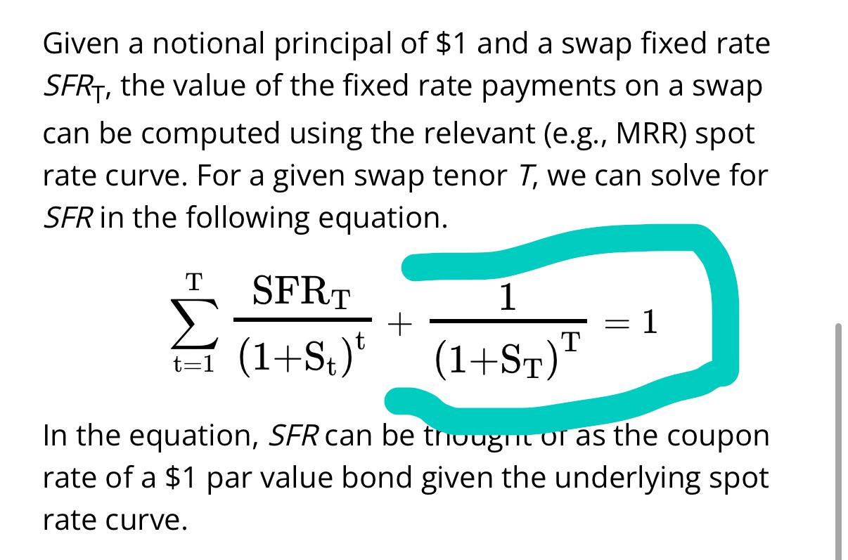
Swap Fixed Rate

Binominal Tree Node distance

i2,LU = i2,LL e^2(std)

Basically log 2std

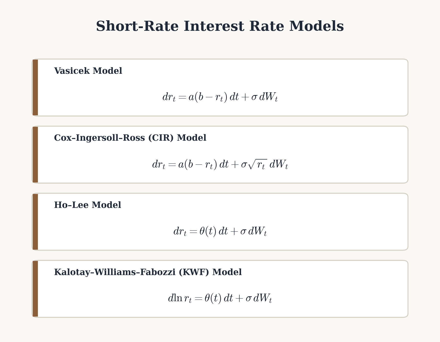
Vasicek, Cox-Ingersoll-Ross, Ho-Lee, KWF Model

Effective Duration

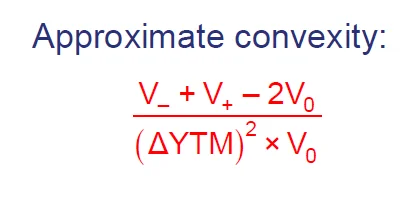
Effective Convexity

Value of Capped and Floored Floater

• Capped

  • Value of straight floater - embedded cap

• Floored

  • Value of straight float - embedded floor

Conversion Value

Market Price of stock * conversion ratio

Market Conversion Price

Market Conversion Premium Ratio

Premium over Straight

Expected Exposure

NPV @ Rfr

• unpaid CF balance

Loss Given Default

Loss Severity * Exposure

Probability of Survival

(1 - Hazard Rate)^t

• Hazard Rate = P(default | no default)

Probability of Default

hazard rate * PS(t-1)

Expected Loss

LGD ( PD

CVA (2 methods)

• Price of rf - Price of risky bond

• PV of Expected Loss of each period

CDS Payout

Notional - MV of CTD bond

payout amount = (1-rr) * notional principal

CDS Spread w/ RR and POD

(1-RR) * POD

Initial payment of CDS

PV(protection leg) - PV(Premium leg)

CDS Spread w/ upfront prem and coupon

Price of CDS per $100 notional

Profit for Protection Buyer

The change in value of a CDS after inception can be approximated by the change in spread multiplied by the duration of the CDS:

profit for protection buyer ≈ change in spread × duration × notional principal

or

profit for protection buyer (%) ≈ change in spread (%) × duration

Equity Forward Price and Value at time T

FP(Equity) = (S0 − PVD) × (1 + Rf)^T = [S0 × (1 + Rf)^T] − FVD

Vt (long) = [St − PVDt] − [FP / (1 + Rf)^(T−t)] = (FPt − FP) / (1 + Rf)^(T−t)

Equity INDEX (forward price)

FP(Equity Index) = S0 × e^((Rf^c − δ^c) × T)

= (S0 × e^(−δ^c × T)) × e^(Rf^c × T)

where: Rf^c = continuously compounded rf = ln(1 + Rf)

δ^c = continuously compounded dividend yield

Fixed Income (forward price)

FP(FI security) = (S0 − PVC) × (1 + Rf)^T

= S0(1 + Rf)^T − FVC

Accrued Interest

Accrued Interest = (days since last coupon payment / days between coupons) × coupon amount

Full price = Clean price + AI

Quoted Forward Price of FI

Quoted FP = FP / CF = [Full price × (1 + Rf)^T − FVC − AI_T] × (1/CF)

FRA Value

([(MRR x d/360) - (contract size x d/360)] x notional)/ (1+ (MRR x d/360))

Swap Fixed Rate

1 - (final discount factor)/sum of all discount factor

discount factor = 1/(1+ [MRR * d/360])

Swap Value to the Payer

Currency Swaps

PV of 2 Cash Flows - Company lended in their local currency

Equity Swap

notional = S1/S0 × $100

prob of up move

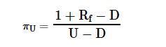
Hedge Ratio

Shares per option

Interest Rate Call/Put Payoff

An interest rate call option has a positive payoff when the reference rate is greater than the exercise rate:

call payoff = notional principal × [Max (0, reference rate − exercise rate)]

Interest rate call options increase in value when rates increase.

An interest rate put option has a positive payoff when the reference rate is less than the exercise rate:

put payoff = notional principal × [Max (0, exercise rate − reference rate)]

BSM for Call/Put No dividends

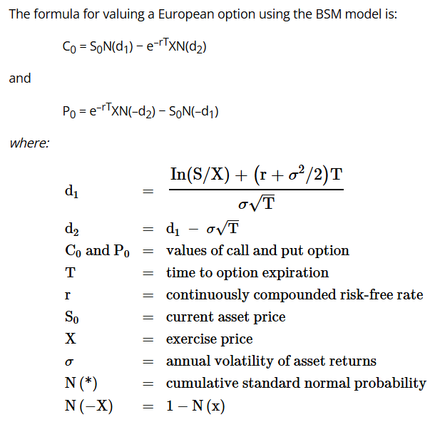
BSM Call/Put for Dividends

BSM Currency Call/Put

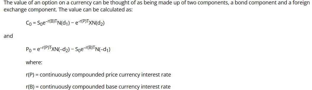
Black Model

For European Futures and Forwards

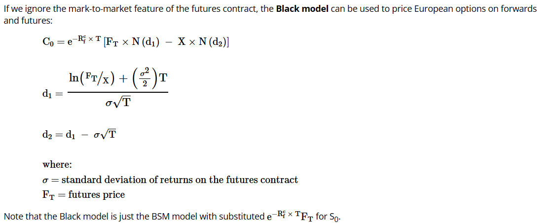
BSM Interest Rate Options

Pay Swaptions

Floors and Caps Values

caplet or floorlet is like an FRA for one period, but with optionality

• Floor = Notional x max(Floor rate - Reference Rate , 0) x days/360

• Caps = Notional x max(Reference Rate - Cap rate, 0) x days/360

Delta

Delta P = Delta - 1

Rho

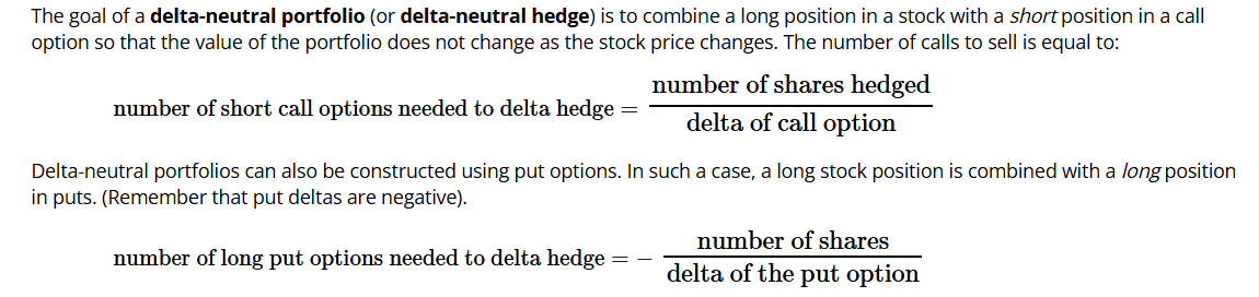
Number of Short Calls to Hedge

Number of Long puts to hedge