Systems Biology and Flux Balance Analysis

• the consumption and production of chemical substances and energy to sustain life

• simple catabolic (breakdown) and anabolic (build up) reactions link together in a sophisticated and coordinated way to convert food into life

what is metabolism

• how cells sense, translate, and respond to external stimuli

• through such reactions cells are able to respond to different chemical and physical signals (e.g. ligands, strains, concentration gradients)

• the response triggered will often be manifested by shifts in gene regulation (control of the levels of enzyme and other proteins via the regulation and control of transcription and translation of the genetic code) in some form

what is signal transduction

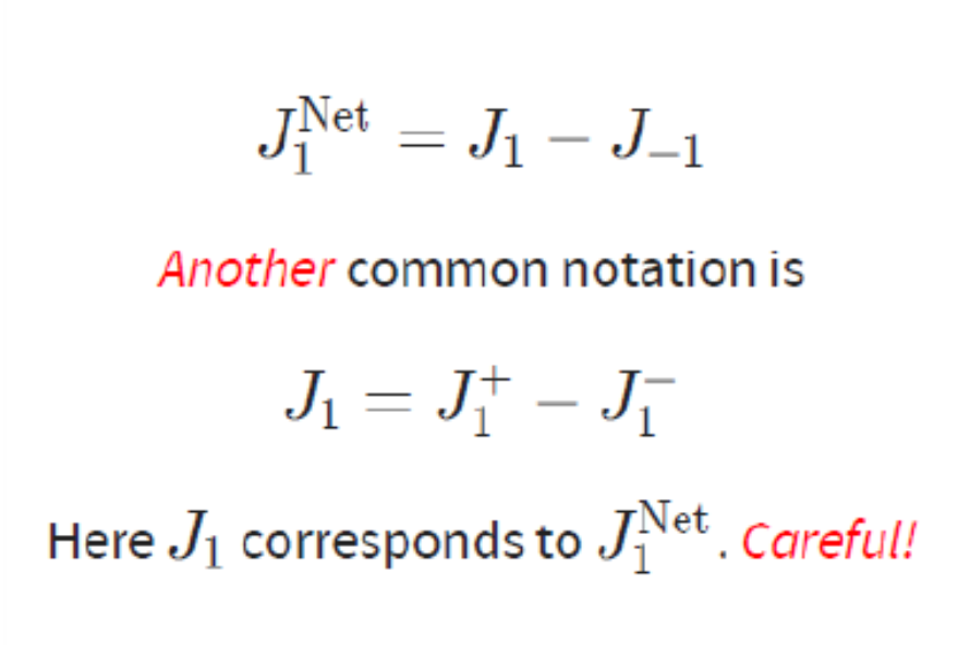
forward reaction - reverse reaction

what is the net flux for a given reaction

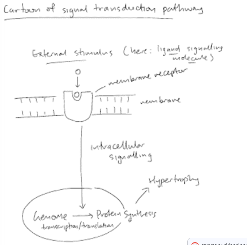
• Heart cells adapt in response to signals reveiced from the rest of the body. One particular response is the increase in cell volume (hypertrophy). This can be a non-pathological adaptation (i.e. in athletes and pregnant mothers). But of more concen is the often pathological, maladaptive case when it can lead to heart disease/failure. 

• We can conceptualise of the signalling process as being initiated by an external stimulus (e.g. a ligand) that binds to a membrane receptor. The receptor initiates a signalling cascade that results in a change in genome regulation. 

Cardiac hypertrophy

• agonist — ligand that stimulates/activates

• antagonist — ligand that blocks action of an agonist

agonist and antagonist ligands

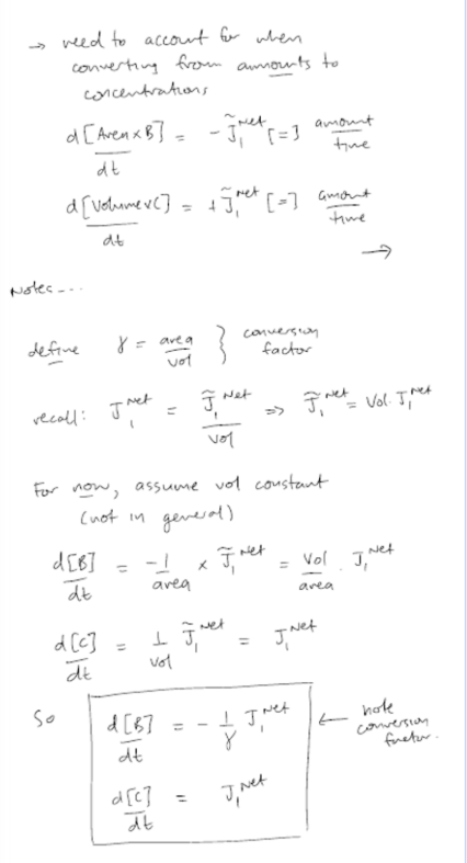
• Core Problem: Chemical reactions conserve total amount (moles/molecules), not concentration. Standard cytosolic reaction models assume a fixed 3D volume, allowing concentration (mol/L or mol/m³) to serve as a proxy for amount

• Dimensional Mismatch: Membrane receptors exist on a 2D surface, making their concentration naturally measured per unit area (mol/m²). Cytosolic species are measured per unit volume (mol/m³)

• Solution: To integrate membrane surface reactions with cytosolic volume reactions while maintaining dimensional consistency, introduce a geometric conversion factor (surface area-to-volume ratio, A/V)

Technical Issue I: Membrane vs Cytosolic Concentration

• Core Problem: Standard Michaelis-Menten (MM) kinetics often assume a constant, static total enzyme concentration (E_T or E₀) over time. However, in complex biological systems — such as those involving transcriptional regulation or signal transduction — enzyme production and degradation continuously alter total enzyme levels in the cytosol.

• Impact on Kinetics: Because maximum reaction velocity is directly proportional to total enzyme (V_max​=k_cat​⋅[E_T​]), fluctuations in enzyme concentration directly shift V_max over time rather than keeping it at a fixed parameter value.

• Solution: Modify standard MM rate equations to treat total enzyme (E(t) or current amount present) rather than a fixed initial constant (E₀)

Technical Issue II: Varying Enzyme Levels

• given a set of parameters and initial conditions, predict the future state of a system

• typically modelling deals with forward problems of this type

Forward problems

• given the measurements of the state of a system, estimate parameters that govern the development of the system and predict future data

• Real-World Context: Represents the primary challenge in empirical science—we can measure system outputs, but determining the exact governing dynamics or predicting outcome under novel conditions is difficult

Inverse problems

The challenge faced by inverse problems is that they may be ill-posed problems with:

• no solution

• many solutions

• unique but unstable solutions

We must persevere despite these challenges. We may draw our attention to other aspects to guide our investigation

• Identifiability and falsifiability — what is possible to learn about how the world works (at a scientific or philosophical level)

• prediction — without understanding the system, can we do something useful such as make predictions (this is the essence of machine learning)

• preferences — we can explicitly warp the system around a model that isn’t necessarily true or useful, but is convenient and comfortable (e.g. consulting)

Ill-posed problems

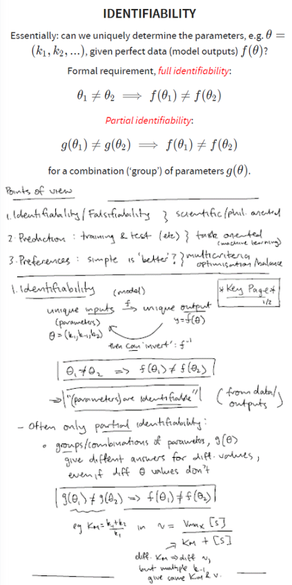
• Core Concept: Determines whether a unique set of model parameters (a={k1​,k2​,…}) can be definitively calculated from perfect model output data f(a).

• Mathematical Definition: a1​=/= a2​⟹f(a1​) =/= f(a2​). Different parameter inputs must produce distinct model outputs for the system to be fully identifiable.

• Examples:

  • Fully Identifiable: y=f(x)=x+1 (every output y corresponds to exactly one input x).

  • Non-Identifiable: y=f(x)=x2 (an output of 4 could come from x=2 or x=−2).

Partial Identifiability: Often, individual parameters cannot be uniquely identified, but specific combinations or groups of parameters (g(a)) can be.

• Biological Context: In Michaelis-Menten kinetics, individual rate constants (k1​,k−1​,kcat​) may yield identical overall reaction velocities under different combinations. However, the parameter grouping K_M​=k_−1​+k_cat/k₁​​ maintains an identifiable relationship with reaction velocity

Identifiability

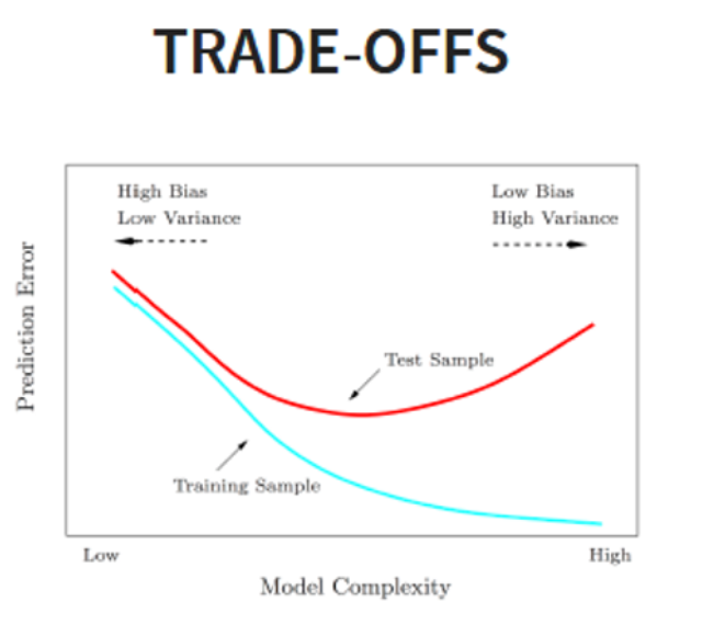
• One key to solving ill-posed problems is recognising the trade-offs involved

  • fit vs complexity — higher-complexity models fit observed data more complexity, but simpler models generalise better

  • overfitting vs underfitting — overfitting captures noise as structural patterns; underfitting fails to capture underlying system dynamics

  • training vs test — optimising model performance exclusively on training data often degrades performance on unseen test data

  • efficiency vs stability — computational speed often comes at the expense of numerical robustness and model stability

  • bias vs variance — high-bias models make strong assumptions and underfit; high-variance models are overly sensitive to small fluctuations in training data

  • etc.

• These trade-offs are closely related and recur throughout science, statistics and engineering

Trade-offs: Prediction and preferences

• core purpose: to systemically measure and quantify how well a mathematical or biological model’s predictions align with experimental data

• key mechanism: utilises a numeric metric — such as norm, distance metric, or cost function (e.g., sum of squared errors) — to calculate model performance

• role in optimisation: providing a single numeric value for performance allows automated algorithms to iteratively adjust parameters to find the optimal fit for the data

evaluating model fit

• Definition: A stoichiometric approach to mathematical modeling that applies the law of conservation of mass to track the net movement (fluxes) of metabolites through complex reaction networks.

• Core Purpose: Enables the study of large-scale metabolic networks (reconstructed from genome sequencing) without needing dynamic rate equations, constitutive laws, or kinetic constants.

• Stoichiometric Matrix (S):

  • Expresses the system of reaction equations in a condensed matrix form by separating reaction flux terms from their coefficients.

  • Captures how species concentrations change across specific reactions in the system.

• Steady State Assumption: Systems are typically analyzed at steady state (dC/dt​=S⋅v=0), representing homeostatic conditions where metabolite concentrations remain constant over time.

• Underdetermined Systems ("The Catch"):

  • Metabolic networks typically feature more reactions/fluxes (columns) than species/metabolites (rows).

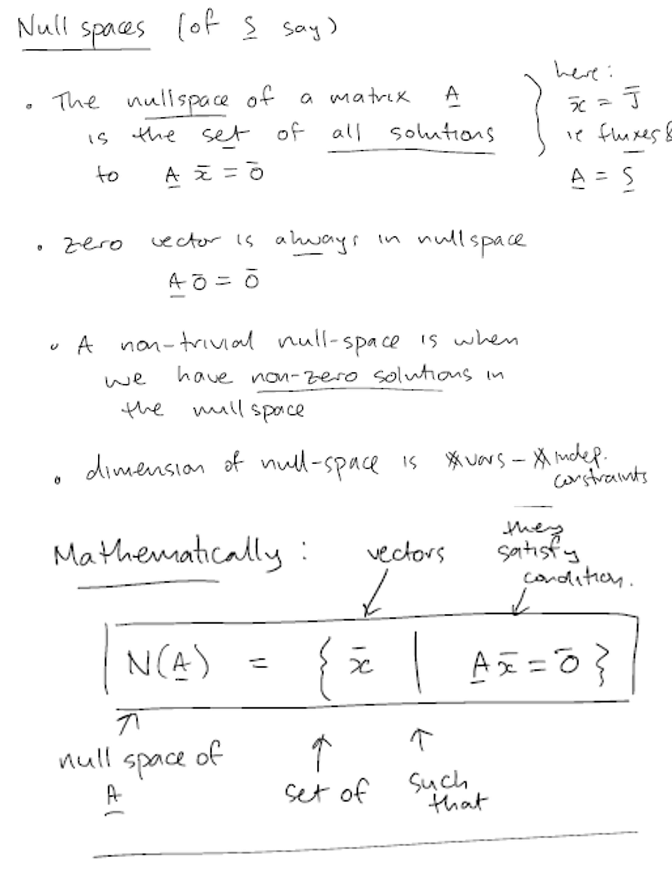
  • This creates an underdetermined system of equations with multiple feasible solutions (a non-trivial null space), requiring optimization methods to resolve.

Flux Balance Analysis

• Underdetermined Nature: Because metabolic networks contain more unknown fluxes than species mass-balance equations, the system has no single unique solution.

• Null Space Representation: The set of all feasible steady-state solutions forms a vector space known as the null space (N(S)). This solution set is expressed as the span (all linear combinations) of a set of linearly independent basis vectors.

• Degrees of Freedom: Each degree of freedom (Ncols​−Nrows​) corresponds to one independent vector in the solution set.

• Finding Solution Vectors: Determine the unique contribution of each free variable by setting it to 1 while setting all other free variables to 0.

• 4-Step Procedure to Solve:

  1. Reduce the stoichiometric matrix S to a minimal set of equations with linearly independent rows.

  2. Select the free variables (count = Ncols​−Nrows​).

  3. Solve for the implied set of independent solution vectors.

  4. Write the final null space solution as N(S)=Span{v1​,v2​,…}.

Solving Metabolic Networks

At this point there are multiple compatible solutions. We can explore these further by:

• Adding bounds (capacity constraints) on fluxes

• Adding directional constraints (from thermodynamics)

• Looking for special 'optimal' solutions (e.g. maximum ATP production)

*FBA is a constraint based analysis in itself ( the constraint being conservation of mass...)

Constraint-based Analysis

• Core Purpose: Transforms constraint-based metabolic modeling into a standard mathematical optimization problem—typically solved using Linear Programming (LP).

• Objective Function (Z or f(v)):

  • Defines the biological or physical goal to be optimized (e.g., Z=c^Tv).

  • Quantified using a linear weight vector (c) that selects or emphasizes specific target fluxes (such as maximizing growth/biomass rate, ATP production, or minimizing byproduct formation).

• Mathematical Formulation:

  • Objective: Maximize or Minimize Z=∑c_i​v_i​

  • Subject to Mass Balance: S⋅v=0 (steady-state stoichiometric constraints)

  • Subject to Flux Bounds: l_i​≤v_i​≤u_i​ (capacity constraints and thermodynamic irreversibility)

• Optimization Output: Identifies a single, mathematically optimal flux vector (v∗) from within the bounded solution space that yields the maximum possible value for the objective function.

General Optimisation Framework