W5 - Poisson regression

Normal distribution parameters

1. mean

2. standard deviation

Poisson distribution parameters

one parameter: lambda (the mean and variance of the poisson distribution)

Outcome variable types - Poisson distribution

• count outcome variables

• discrete positive integers

as lambda increases the distribution …

begins to look more similar to a normal distribution

Why linear regression cannot be used for count data

• The normality distribution would be violated (unless high avg counts)'

• Can't have negative numbers

• Certainty at extreme values is impossible when the outcome can only be 0 or positive whole numbers

• when an outcome can only be 0 or positive whole numbers, a straight line is a bad fit, and is impossible for extreme values (negative)

Solution: link function

• resolves the issue of count data not having negative values

• the link function transforms the linear predicted value η so that it never goes below zero

Group comparisons

poisson and logistic regression used z-scores rather than t-values

Link function for poisson regression

η = g(λ) = ln(λ)

Takes the average number of counts (lambda), which can only fall > 0, and transforms it to fall between negative infinity and positive infinity. This gives us a continuous and unbounded outcome we can apply a linear model to.

• natural log transformation unbounds lambda on the left side of the graph so that it never goes below zero

• log of zero = negative infinity (cannot go under zero)

ln()

the natural logarithm (or log with base e, euler's number)

Poisson regression

• Used when the outcome is a count variable (discrete, whole and positive)

• Poisson distribution used when the counts are relatively rare

• Poisson distribution: discrete, density curve not plotted

• Only has one distribution parameter - Lambda (mean + variance)

• As lambda increases may start to look more like a normal distribution

Inverse link function

reverts predictions made from linear model back to original count scale so predictions can be interpreted

• transforms eta back to fall > 0

Poisson regression assumptions

• assumes a poisson distribution

• errors are independent

• assumes that on the link scale (natural log scale) there is a linear relationship

• assumptions of equal variance and normality not required

• Requires a large sample size. There are no degrees of freedom so sample must be large enough that parameters are distributed about normally relying on the central limit theorem

*no agreed upon method for evaluating whether residual meet assumptions

Poisson regression in R

• Use glm() function

• When using anything other than a linear model need to specify family argument e.g. family = poisson()

• m <- glm(num_awards ~ math, data = dcount, family = poisson())

Poisson output

• Deviance residuals: how much each data point contributed to the residual deviance. Measure of overall model fit. Not calculated as the raw difference between each data point and predicted value.

• Coefficients: z-values instead of t-values as we cannot calculate degrees of freedom

• No R2 - only works for linear regression. Instead get the null and residual deviance values and an AIC (relative measure of model fit taking into account model complexity)

• Number of Fisher scoring iterations

Poisson regression interpretation

A poisson regression predicting the number of awards each student received from their math scores showed that students who had a 0 math score were expected to have -5.33 log awards, p < .001. Each one unit higher math score was associated with 0.09 higher log awards, p < .001. A graph of these results follows.

 - by specifying that we are working on a log scale can interpret the results as we did before

• hard to interpret results on log scale

Incident rate ratios

• Obtained by exponentiating the regression coefficients (slopes)

  *can exp coefficients & confint, but not p-values or z-values

• IRRs indicate how many more times the outcome will be for a one unit change in the predictor

• e.g. if the IRR=2  and the base rate was 1, then one unit higher would be 1∗2=2. If the base rate was 2, then a one unit higher would be 2∗2=4

• IRRs are interpreted as for each one unit higher predictor score, there are IRR times as many events of the outcome.

• How much your outcome is expected to increase in count numbers

• As IRRs are multiplicative, an IRR of 1 means that a one unit change in the predictor is associated with 1 times as many events on the outcome, that is no change.

• On the IRR scale, a coefficient of 1 is equivalent to a coefficient of 0 on the link (log) scale

Interpretation using IRRs

A poisson regression predicting the number of awards each student received from their math scores showed that students who had a 0 math score were expected to have 0.00 awards, [95% CI 0.00 - 0.01]. Each one unit higher math score was associated with having 1.09 times the number of awards, [95% CI 1.07 - 1.11], p < .001. A graph of these results follows.

eta

expected part of the model without error term

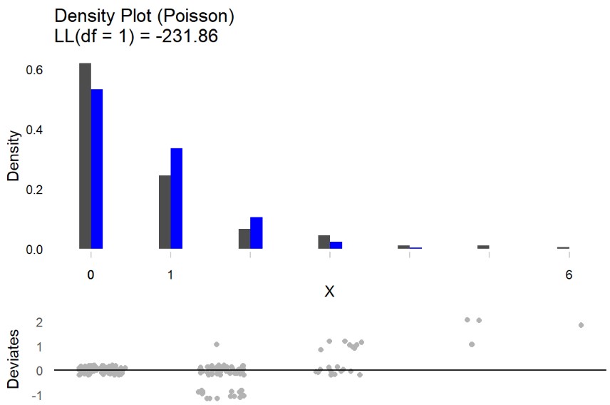
Poisson testDistribution()

discrete distribution

• solid grey bars show the observed density of different values

• blue bars show the density under a poisson distribution

• deviates plot show the deviations from the assumed poisson distribution